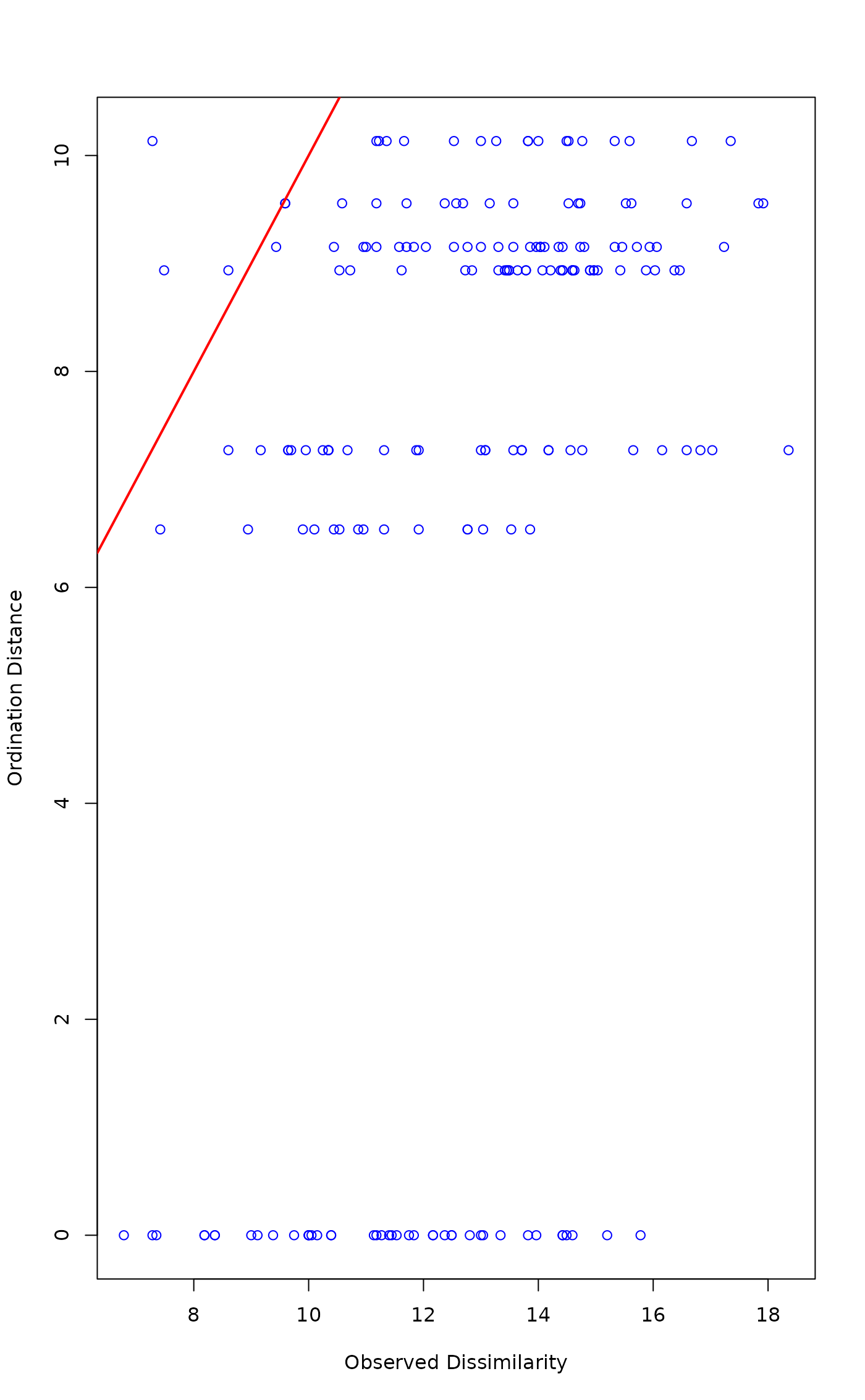
Display Ordination Distances Against Observed Distances in Eigenvector Ordinations

Functions plot ordination distances in given number of dimensions against observed distances or distances in full space in eigenvector methods. The display is similar as the Shepard diagram (stressplot for non-metric multidimensional scaling with metaMDS or monoMDS), but shows the linear relationship of the eigenvector ordinations. The stressplot methods are available for wcmdscale, rda, cca, capscale, dbrda, prcomp and princomp.

Usage

# S3 method for class 'wcmdscale'
stressplot(object, k = 2, pch, p.col = "blue", l.col = "red",
    lwd = 2, ...)

Arguments

object: Result object from eigenvector ordination (wcmdscale, rda, cca, dbrda, capscale)
k: Number of dimensions for which the ordination distances are displayed.
pch, p.col, l.col, lwd: Plotting character, point colour and line colour like in default stressplot
...: Other parameters to functions, e.g. graphical parameters.

Details

The functions offer a similar display for eigenvector ordinations as the standard Shepard diagram (stressplot) in non-metric multidimensional scaling. The ordination distances in given number of dimensions are plotted against observed distances. With metric distances, the ordination distances in full space (with all ordination axes) are equal to observed distances, and the fit line shows this equality. In general, the fit line does not go through the points, but the points for observed distances approach the fit line from below. However, with non-Euclidean distances (in wcmdscale, dbrda or capscale) with negative eigenvalues the ordination distances can exceed the observed distances in real dimensions; the imaginary dimensions with negative eigenvalues will correct these excess distances. If you have used dbrda, capscale or wcmdscale with argument add to avoid negative eigenvalues, the ordination distances will exceed the observed dissimilarities.

In partial ordination (cca, rda, and capscale with Condition in the formula), the distances in the partial component are included both in the observed distances and in ordination distances. With k=0, the ordination distances refer to the partial ordination. The exception is dbrda where the distances in partial, constrained and residual components are not additive, and only the first of these components can be shown, and partial models cannot be shown at all.

Value

Functions draw a graph and return invisibly the ordination distances or the ordination distances.

Author

Jari Oksanen.

Examples

data(dune, dune.env)
mod <- rda(dune)
stressplot(mod)

mod <- rda(dune ~ Management, dune.env)
stressplot(mod, k=3)