Nonmetric Multidimensional Scaling with Stable Solution from Random Starts, Axis Scaling and Species Scores

Function metaMDS performs Nonmetric Multidimensional Scaling (NMDS), and tries to find a stable solution using several random starts. In addition, it standardizes the scaling in the result, so that the configurations are easier to interpret, and adds species scores to the site ordination. The metaMDS function does not provide actual NMDS, but it calls another function for the purpose. Currently monoMDS is the default choice, but it is also possible to call other functions as an engine.

Usage

metaMDS(comm, distance = "bray", k = 2, try = 20, trymax = 20, 
    engine = monoMDS, autotransform =TRUE, noshare = FALSE, wascores = TRUE,
    expand = TRUE, trace = 1, plot = FALSE, previous.best,  ...)
# S3 method for class 'metaMDS'
plot(x, display = c("sites", "species"), choices = c(1, 2),
    type = "p", shrink = FALSE, cex = 0.7, ...)
# S3 method for class 'metaMDS'
points(x, display = c("sites", "species"),
    choices = c(1,2), shrink = FALSE, select, cex = 0.7, ...)
# S3 method for class 'metaMDS'
text(x, display = c("sites", "species"), labels, 
    choices = c(1,2), shrink = FALSE, select, cex = 0.7, ...)
# S3 method for class 'metaMDS'
scores(x, display = c("sites", "species"), shrink = FALSE, 
    choices, tidy = FALSE, ...)
metaMDSdist(comm, distance = "bray", autotransform = TRUE, 
    noshare = TRUE, trace = 1, commname, zerodist = "ignore", 
    distfun = vegdist, ...)
metaMDSiter(dist, k = 2, try = 20, trymax = 20, trace = 1, plot = FALSE, 
    previous.best, engine = monoMDS, maker, parallel = getOption("mc.cores"),
    ...)
initMDS(x, k=2)
postMDS(X, dist, pc=TRUE, center=TRUE, halfchange, threshold=0.8,
    nthreshold=10, plot=FALSE, ...)
metaMDSredist(object, ...)

Arguments

comm: Community data. Alternatively, dissimilarities either as a dist structure or as a symmetric square matrix. In the latter case all other stages are skipped except random starts and centring and pc rotation of axes.
distance: Dissimilarity index used in vegdist.
k: Number of dimensions. NB., the number of points \(n\) should be \(n > 2k + 1\), and preferably much higher in global non-metric MDS, and still higher in local NMDS.
try, trymax: Minimum and maximum numbers of random starts in search of stable solution. After try has been reached, the iteration will stop when similar solutions were repeated or trymax was reached.
engine: The function used for MDS. The default is to use the monoMDS function in vegan. It is also possible to use any MDS function which takes as three first arguments (in this order) input dissimilarities, matrix of initial configuration and number of dimensions, and returns a list with items stress and points for final configuration. See Examples for wrapping a compatible function.
autotransform: Use simple heuristics for possible data transformation of typical community data (see below). If you do not have community data, you should probably set autotransform = FALSE.
noshare: Triggering of calculation step-across or extended dissimilarities with function stepacross. The argument can be logical or a numerical value greater than zero and less than one. If TRUE, extended dissimilarities are used always when there are no shared species between some sites, if FALSE, they are never used. If noshare is a numerical value, stepacross is used when the proportion of site pairs with no shared species exceeds noshare. The number of pairs with no shared species is found with no.shared function, and noshare has no effect if input data were dissimilarities instead of community data.
wascores: Calculate species scores using function wascores.
expand: Expand weighted averages of species in wascores.
trace: Trace the function; trace = 2 or higher will be more voluminous.
plot: Graphical tracing: plot interim results. You may want to set par(ask = TRUE) with this option.
previous.best: Start searches from a previous solution. This can also be a monoMDS solution or a matrix of coordinates.
x: metaMDS result (or a dissimilarity structure for initMDS).
choices: Axes shown.
type: Plot type: "p" for points, "t" for text, and "n" for axes only.
display: Display "sites" or "species".
shrink: Shrink back species scores if they were expanded originally.
cex: Character expansion for plotting symbols.
tidy: Return scores that are compatible with ggplot2: all scores are in a single data.frame, score type is identified by factor variable code ("sites" or "species"), the names by variable label. These scores are incompatible with conventional plot functions, but they can be used in ggplot2.
labels: Optional test to be used instead of row names. If select is used, labels are given only to selected items in the order they occur in the scores.
select: Items to be displayed. This can either be a logical vector which is TRUE for displayed items or a vector of indices of displayed items.
X: Configuration from multidimensional scaling.
commname: The name of comm: should not be given if the function is called directly.
zerodist: Handling of zero dissimilarities: either "fail" or "add" a small positive value, or "ignore". monoMDS and many other functions accept zero dissimilarities and the default is zerodist = "ignore", but with isoMDS you may need to set zerodist = "add".
distfun: Dissimilarity function. Any function returning a dist object and accepting argument method can be used (but some extra arguments may cause name conflicts).
maker: The name (character) of the engine. Only "monoMDS" has an effect and triggers some actions that are not known to be available with other engines.
parallel: Number of parallel processes or a predefined socket cluster. If you use pre-defined socket clusters (say, clus), you must issue clusterEvalQ(clus, library(vegan)) to make available internal vegan functions. With parallel = 1 uses ordinary, non-parallel processing. The parallel processing is done with parallel package.
dist: Dissimilarity matrix used in multidimensional scaling.
pc: Rotate to principal axes.
center: Centre the configuration.
halfchange: Scale axes to half-change units. This defaults TRUE when dissimilarities are known to have a theoretical maximum value (ceiling). Function vegdist will have that information in attribute maxdist, and for other distfun this is interpreted in a simple test (that can fail), and the information may not available when input data are distances. If FALSE, the ordination dissimilarities are scaled to the same range as the input dissimilarities.
threshold: Largest dissimilarity used in half-change scaling. If dissimilarities have a known (or inferred) ceiling, threshold is relative to that ceiling (see halfchange).
nthreshold: Minimum number of points in half-change scaling.
object: A result object from metaMDS.
...: Other parameters passed to functions. Function metaMDS passes all arguments to its component functions metaMDSdist, metaMDSiter, postMDS, and to distfun and engine.

Details

Non-metric Multidimensional Scaling (NMDS) is commonly regarded as the most robust unconstrained ordination method in community ecology (Minchin 1987). Function metaMDS is a wrapper function that calls several other functions to combine Minchin's (1987) recommendations into one command. The complete steps in metaMDS are:

Transformation: If the data values are larger than common abundance class scales, the function performs a Wisconsin double standardization (wisconsin). If the values look very large, the function also performs sqrt transformation. Both of these standardizations are generally found to improve the results. However, the limits are completely arbitrary (at present, data maximum 50 triggers sqrt and \(>9\) triggers wisconsin). If you want to have a full control of the analysis, you should set autotransform = FALSE and standardize and transform data independently. The autotransform is intended for community data, and for other data types, you should set autotransform = FALSE. This step is perfomed using metaMDSdist, and the step is skipped if input were dissimilarities.
Choice of dissimilarity: For a good result, you should use dissimilarity indices that have a good rank order relation to ordering sites along gradients (Faith et al. 1987). The default is Bray-Curtis dissimilarity, because it often is the test winner. However, any other dissimilarity index in vegdist can be used. Function rankindex can be used for finding the test winner for you data and gradients. The default choice may be bad if you analyse other than community data, and you should probably select an appropriate index using argument distance. This step is performed using metaMDSdist, and the step is skipped if input were dissimilarities.
Step-across dissimilarities: Ordination may be very difficult if a large proportion of sites have no shared species. In this case, the results may be improved with stepacross dissimilarities, or flexible shortest paths among all sites. The default NMDS engine is monoMDS which is able to break tied values at the maximum dissimilarity, and this is usually sufficient to handle cases with no shared species. stepacross is triggered by option noshare. If you do not like manipulation of original distances, you should set noshare = FALSE. This step is performed using metaMDSdist, and the step is skipped always when input were dissimilarities.
NMDS with random starts: NMDS easily gets trapped into local optima, and you must start NMDS several times from random starts to be confident that you have found the global solution. The strategy in metaMDS is to first run NMDS starting with the metric scaling (cmdscale which usually finds a good solution but often close to a local optimum), or use the previous.best solution if supplied, and take its solution as the standard (Run 0). Then metaMDS starts NMDS from several random starts (minimum number is given by try and maximum number by trymax). These random starts are generated by initMDS. If a solution is better (has a lower stress) than the previous standard, it is taken as the new standard. If the solution is better or close to a standard, metaMDS compares two solutions using Procrustes analysis (function procrustes with option symmetric = TRUE). If the solutions are very similar in their Procrustes rmse and the largest residual is very small, the solutions are regarded as repeated and the better one is taken as the new standard. The conditions are stringent, and you may have found good and relatively similar solutions although the function is not yet satisfied. Setting trace = TRUE will monitor the final stresses, and plot = TRUE will display Procrustes overlay plots from each comparison. This step is performed using metaMDSiter. This is the first step performed if input data (comm) were dissimilarities. Random starts can be run with parallel processing (argument parallel).
Scaling of the results: metaMDS will run postMDS for the final result. Function postMDS provides the following ways of “fixing” the indeterminacy of scaling and orientation of axes in NMDS: Centring moves the origin to the average of the axes; Principal components rotate the configuration so that the variance of points is maximized on first dimension (with function MDSrotate you can alternatively rotate the configuration so that the first axis is parallel to an environmental variable); Half-change scaling scales the configuration so that one unit means halving of community similarity from replicate similarity. Half-change scaling is based on closer dissimilarities where the relation between ordination distance and community dissimilarity is rather linear (the limit is set by argument threshold). If there are enough points below this threshold (controlled by the parameter nthreshold), dissimilarities are regressed on distances. The intercept of this regression is taken as the replicate dissimilarity, and half-change is the distance where similarity halves according to linear regression. Obviously the method is applicable only for dissimilarity indices scaled to \(0 \ldots 1\), such as Kulczynski, Bray-Curtis and Canberra indices. If half-change scaling is not used, the ordination is scaled to the same range as the original dissimilarities. Half-change scaling is skipped by default if input were dissimilarities, but can be turned on with argument halfchange = TRUE. NB., The PC rotation only changes the directions of reference axes, and it does not influence the configuration or solution in general.
Species scores: Function adds the species scores to the final solution as weighted averages using function wascores with given value of parameter expand. The expansion of weighted averages can be undone with shrink = TRUE in plot or scores functions, and the calculation of species scores can be suppressed with wascores = FALSE. This step is skipped if input were dissimilarities and community data were unavailable. However, the species scores can be added or replaced with sppscores.

Results Could Not Be Repeated

Non-linear optimization is a hard task, and the best possible solution (“global optimum”) may not be found from a random starting configuration. Most software solve this by starting from the result of metric scaling (cmdscale). This will probably give a good result, but not necessarily the “global optimum”. Vegan does the same, but metaMDS tries to verify or improve this first solution (“try 0”) using several random starts and seeing if the result can be repeated or improved and the improved solution repeated. If this does not succeed, you get a message that the result could not be repeated. However, the result will be at least as good as the usual standard strategy of starting from metric scaling or it may be improved. You may not need to do anything after such a message, but you can be satisfied with the result. If you want to be sure that you probably have a “global optimum” you may try the following instructions.

With default engine = "monoMDS" the function will tabulate the stopping criteria used, so that you can see which criterion should be made more stringent. The criteria can be given as arguments to metaMDS and their current values are described in monoMDS. In particular, if you reach the maximum number of iterations, you should increase the value of maxit. You may ask for a larger number of random starts without losing the old ones giving the previous solution in argument previous.best.

In addition to slack convergence criteria and too low number of random starts, wrong number of dimensions (argument k) is the most common reason for not being able to repeat similar solutions. NMDS is usually run with a low number dimensions (k=2 or k=3), and for complex data increasing k by one may help. If you run NMDS with much higher number of dimensions (say, k=10 or more), you should reconsider what you are doing and drastically reduce k. For very heterogeneous data sets with partial disjunctions, it may help to set stepacross, but for most data sets the default weakties = TRUE is sufficient.

Please note that you can give all arguments of other metaMDS* functions and NMDS engine (default monoMDS) in your metaMDS command,and you should check documentation of these functions for details.

Common Wrong Claims

NMDS is often misunderstood and wrong claims of its properties are common on the Web and even in publications. It is often claimed that the NMDS configuration is non-metric which means that you cannot fit environmental variables or species onto that space. This is a false statement. In fact, the result configuration of NMDS is metric, and it can be used like any other ordination result. In NMDS the rank orders of Euclidean distances among points in ordination have a non-metric monotone relationship to any observed dissimilarities. The transfer function from observed dissimilarities to ordination distances is non-metric (Kruskal 1964a, 1964b), but the ordination result configuration is metric and observed dissimilarities can be of any kind (metric or non-metric).

The ordination configuration is usually rotated to principal axes in metaMDS. The rotation is performed after finding the result, and it only changes the direction of the reference axes. Before rotation the directions of axes are arbitrary, and the same solution (same configuration, same stress) the orientation of axes is arbitrary. The only important feature in the NMDS solution are the ordination distances, and these do not change in rotation. Similarly, the rank order of distances does not change in uniform scaling or centring of configuration of points. You can also rotate the NMDS solution to external environmental variables with MDSrotate. This rotation will also only change the orientation of axes, but will not change the configuration of points or distances between points in ordination space.

Function stressplot displays the method graphically: it plots the observed dissimilarities against distances in ordination space, and also shows the non-metric monotone regression.

Value

Function metaMDS returns an object of class metaMDS which inherits from the class of engine. The final site ordination is stored in the item points, and species ordination in the item species, and the stress in item stress (NB, the scaling of the stress depends on the engine: isoMDS uses percents, monoMDS and most other functions use proportions \(0 \ldots 1\)). The other items store the information on the steps taken and the items returned by the engine function. The object has print, plot, points and text methods. Functions metaMDSdist and metaMDSredist return vegdist objects. Function initMDS returns a random configuration. Functions metaMDSiter and postMDS returns the result of NMDS with updated configuration.

References

Faith, D. P, Minchin, P. R. and Belbin, L. (1987). Compositional dissimilarity as a robust measure of ecological distance. Vegetatio 69, 57–68.

Kruskal, J.B. (1964a). Multidimensional scaling by optimizing goodness-of-fit to a nonmetric hypothesis. Psychometrika 29, 1–28.

Kruskal, J.B. (1964b). Nonmetric multidimensional scaling: a numerical method. Psychometrika 29, 115–129.

Minchin, P.R. (1987). An evaluation of relative robustness of techniques for ecological ordinations. Vegetatio 69, 89–107.

Author

Jari Oksanen

Note

Function metaMDS is a simple wrapper for an NMDS engine (either monoMDS or any compatible function, and some support functions (metaMDSdist, stepacross, metaMDSiter, initMDS, postMDS, wascores). You can call these support functions separately for the full control of results. Data transformation, dissimilarities and possible stepacross are made in function metaMDSdist which returns a dissimilarity result. Iterative search (with starting values from initMDS with selected engine is made in metaMDSiter. Post-processing of result configuration is done in postMDS, and species scores added by wascores. If you want to be more certain of reaching a global solution, you can compare results from several independent runs. You can also continue analysis from previous results or from your own configuration. Function may not save the used dissimilarity matrix (monoMDS does), but metaMDSredist tries to reconstruct the used dissimilarities with original data transformation and possible stepacross.

The metaMDS function was designed to be used with community data. If you have other type of data, you should probably set some arguments to non-default values: probably at least wascores, autotransform and noshare should be FALSE. If you have negative data entries, metaMDS will set the previous to FALSE with a warning.

Examples

## The recommended way of running NMDS (Minchin 1987)
##
data(dune)
## IGNORE_RDIFF_BEGIN
## Global NMDS using monoMDS
sol <- metaMDS(dune)
#> Run 0 stress 0.1192678 
#> Run 1 stress 0.1183186 
#> ... New best solution
#> ... Procrustes: rmse 0.02027016  max resid 0.06496137 
#> Run 2 stress 0.1183186 
#> ... Procrustes: rmse 2.410807e-05  max resid 5.016223e-05 
#> ... Similar to previous best
#> Run 3 stress 0.1183186 
#> ... Procrustes: rmse 1.38321e-06  max resid 4.005019e-06 
#> ... Similar to previous best
#> Run 4 stress 0.1809577 
#> Run 5 stress 0.1183186 
#> ... Procrustes: rmse 1.298239e-05  max resid 4.209378e-05 
#> ... Similar to previous best
#> Run 6 stress 0.1183186 
#> ... Procrustes: rmse 8.687808e-06  max resid 2.812715e-05 
#> ... Similar to previous best
#> Run 7 stress 0.1901489 
#> Run 8 stress 0.1192678 
#> Run 9 stress 0.1192678 
#> Run 10 stress 0.1192678 
#> Run 11 stress 0.1192678 
#> Run 12 stress 0.1183186 
#> ... Procrustes: rmse 4.96679e-06  max resid 1.631071e-05 
#> ... Similar to previous best
#> Run 13 stress 0.1886532 
#> Run 14 stress 0.1183186 
#> ... Procrustes: rmse 8.559538e-06  max resid 2.016705e-05 
#> ... Similar to previous best
#> Run 15 stress 0.1183186 
#> ... Procrustes: rmse 2.670719e-06  max resid 7.850138e-06 
#> ... Similar to previous best
#> Run 16 stress 0.2035424 
#> Run 17 stress 0.1808911 
#> Run 18 stress 0.1808911 
#> Run 19 stress 0.1183186 
#> ... Procrustes: rmse 2.790912e-06  max resid 8.334662e-06 
#> ... Similar to previous best
#> Run 20 stress 0.1192678 
#> *** Best solution repeated 8 times
sol
#> 
#> Call:
#> metaMDS(comm = dune) 
#> 
#> global Multidimensional Scaling using monoMDS
#> 
#> Data:     dune 
#> Distance: bray 
#> 
#> Dimensions: 2 
#> Stress:     0.1183186 
#> Stress type 1, weak ties
#> Best solution was repeated 8 times in 20 tries
#> The best solution was from try 1 (random start)
#> Scaling: centring, PC rotation, halfchange scaling 
#> Species: expanded scores based on ‘dune’ 
#> 
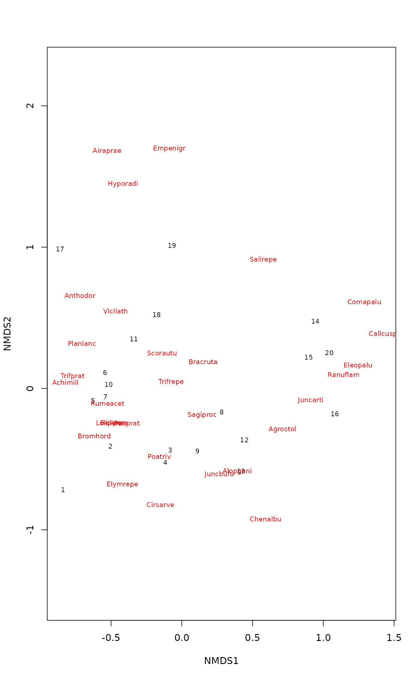
plot(sol, type="t", optimize = TRUE)

## Start from previous best solution
sol <- metaMDS(dune, previous.best = sol)
#> Starting from 2-dimensional configuration
#> Run 0 stress 0.1183186 
#> Run 1 stress 0.1808911 
#> Run 2 stress 0.1183186 
#> ... Procrustes: rmse 3.088594e-06  max resid 9.804563e-06 
#> ... Similar to previous best
#> Run 3 stress 0.1183186 
#> ... Procrustes: rmse 1.663967e-06  max resid 5.755877e-06 
#> ... Similar to previous best
#> Run 4 stress 0.1812933 
#> Run 5 stress 0.1183186 
#> ... Procrustes: rmse 1.099909e-05  max resid 3.500602e-05 
#> ... Similar to previous best
#> Run 6 stress 0.1183186 
#> ... Procrustes: rmse 9.144568e-06  max resid 2.87281e-05 
#> ... Similar to previous best
#> Run 7 stress 0.1192679 
#> Run 8 stress 0.1192678 
#> Run 9 stress 0.1192679 
#> Run 10 stress 0.1183186 
#> ... Procrustes: rmse 3.871203e-06  max resid 1.197668e-05 
#> ... Similar to previous best
#> Run 11 stress 0.1183186 
#> ... Procrustes: rmse 3.732854e-06  max resid 9.038913e-06 
#> ... Similar to previous best
#> Run 12 stress 0.1183186 
#> ... Procrustes: rmse 1.304077e-06  max resid 3.708914e-06 
#> ... Similar to previous best
#> Run 13 stress 0.1183186 
#> ... Procrustes: rmse 3.277354e-06  max resid 1.065231e-05 
#> ... Similar to previous best
#> Run 14 stress 0.1192678 
#> Run 15 stress 0.1192679 
#> Run 16 stress 0.1192678 
#> Run 17 stress 0.1192678 
#> Run 18 stress 0.1183186 
#> ... Procrustes: rmse 1.585904e-05  max resid 5.090747e-05 
#> ... Similar to previous best
#> Run 19 stress 0.1183186 
#> ... Procrustes: rmse 2.684485e-06  max resid 7.322967e-06 
#> ... Similar to previous best
#> Run 20 stress 0.1192679 
#> *** Best solution repeated 18 times
## Local NMDS and stress 2 of monoMDS
sol2 <- metaMDS(dune, model = "local", stress=2)
#> Run 0 stress 0.1928478 
#> Run 1 stress 0.1928479 
#> ... Procrustes: rmse 0.0005674005  max resid 0.001657282 
#> ... Similar to previous best
#> Run 2 stress 0.1928477 
#> ... New best solution
#> ... Procrustes: rmse 5.951658e-05  max resid 0.0001814182 
#> ... Similar to previous best
#> Run 3 stress 0.1928476 
#> ... New best solution
#> ... Procrustes: rmse 3.670919e-05  max resid 0.0001026632 
#> ... Similar to previous best
#> Run 4 stress 0.1928488 
#> ... Procrustes: rmse 0.0006356863  max resid 0.00179782 
#> ... Similar to previous best
#> Run 5 stress 0.1928476 
#> ... New best solution
#> ... Procrustes: rmse 2.606034e-05  max resid 7.248371e-05 
#> ... Similar to previous best
#> Run 6 stress 0.1928478 
#> ... Procrustes: rmse 6.793629e-05  max resid 0.0001527193 
#> ... Similar to previous best
#> Run 7 stress 0.1928476 
#> ... Procrustes: rmse 0.0003387622  max resid 0.0009712344 
#> ... Similar to previous best
#> Run 8 stress 0.1928481 
#> ... Procrustes: rmse 0.00050691  max resid 0.001484753 
#> ... Similar to previous best
#> Run 9 stress 0.1928476 
#> ... New best solution
#> ... Procrustes: rmse 0.0002904976  max resid 0.0008646559 
#> ... Similar to previous best
#> Run 10 stress 0.1928475 
#> ... New best solution
#> ... Procrustes: rmse 5.395683e-05  max resid 0.0001905499 
#> ... Similar to previous best
#> Run 11 stress 0.192848 
#> ... Procrustes: rmse 0.0004562282  max resid 0.001302441 
#> ... Similar to previous best
#> Run 12 stress 0.1928475 
#> ... New best solution
#> ... Procrustes: rmse 0.0001225484  max resid 0.0003602622 
#> ... Similar to previous best
#> Run 13 stress 0.1928475 
#> ... New best solution
#> ... Procrustes: rmse 7.362496e-05  max resid 0.0001729474 
#> ... Similar to previous best
#> Run 14 stress 0.1928482 
#> ... Procrustes: rmse 0.0004090245  max resid 0.001212783 
#> ... Similar to previous best
#> Run 15 stress 0.1928481 
#> ... Procrustes: rmse 0.0003940302  max resid 0.001165363 
#> ... Similar to previous best
#> Run 16 stress 0.1928475 
#> ... Procrustes: rmse 4.177447e-05  max resid 0.0001231291 
#> ... Similar to previous best
#> Run 17 stress 0.1928476 
#> ... Procrustes: rmse 0.0001088397  max resid 0.0003218042 
#> ... Similar to previous best
#> Run 18 stress 0.1928479 
#> ... Procrustes: rmse 0.0003334197  max resid 0.0009563268 
#> ... Similar to previous best
#> Run 19 stress 0.1928481 
#> ... Procrustes: rmse 0.0003993959  max resid 0.001152288 
#> ... Similar to previous best
#> Run 20 stress 0.1928477 
#> ... Procrustes: rmse 0.0002728073  max resid 0.0007940036 
#> ... Similar to previous best
#> *** Best solution repeated 8 times
sol2
#> 
#> Call:
#> metaMDS(comm = dune, model = "local", stress = 2) 
#> 
#> local Multidimensional Scaling using monoMDS
#> 
#> Data:     dune 
#> Distance: bray 
#> 
#> Dimensions: 2 
#> Stress:     0.1928475 
#> Stress type 2, weak ties
#> Best solution was repeated 8 times in 20 tries
#> The best solution was from try 13 (random start)
#> Scaling: centring, PC rotation, halfchange scaling 
#> Species: expanded scores based on ‘dune’ 
#> 
## Use Arrhenius exponent 'z' as a binary dissimilarity measure
sol <- metaMDS(dune, distfun = betadiver, distance = "z")
#> Run 0 stress 0.1067169 
#> Run 1 stress 0.1073148 
#> Run 2 stress 0.107471 
#> Run 3 stress 0.1073148 
#> Run 4 stress 0.1069791 
#> ... Procrustes: rmse 0.006878154  max resid 0.0243509 
#> Run 5 stress 0.1067169 
#> ... New best solution
#> ... Procrustes: rmse 3.557419e-06  max resid 9.05284e-06 
#> ... Similar to previous best
#> Run 6 stress 0.1067169 
#> ... Procrustes: rmse 2.92448e-06  max resid 7.000251e-06 
#> ... Similar to previous best
#> Run 7 stress 0.1067169 
#> ... Procrustes: rmse 5.57065e-06  max resid 1.500797e-05 
#> ... Similar to previous best
#> Run 8 stress 0.1834483 
#> Run 9 stress 0.1069784 
#> ... Procrustes: rmse 0.0067185  max resid 0.02361645 
#> Run 10 stress 0.1067169 
#> ... Procrustes: rmse 2.445873e-06  max resid 6.115258e-06 
#> ... Similar to previous best
#> Run 11 stress 0.1716981 
#> Run 12 stress 0.1067169 
#> ... Procrustes: rmse 1.495835e-05  max resid 3.49344e-05 
#> ... Similar to previous best
#> Run 13 stress 0.107471 
#> Run 14 stress 0.1649904 
#> Run 15 stress 0.1689845 
#> Run 16 stress 0.107471 
#> Run 17 stress 0.1694184 
#> Run 18 stress 0.1742036 
#> Run 19 stress 0.1067169 
#> ... Procrustes: rmse 2.360969e-06  max resid 4.926857e-06 
#> ... Similar to previous best
#> Run 20 stress 0.1073148 
#> *** Best solution repeated 6 times
sol
#> 
#> Call:
#> metaMDS(comm = dune, distance = "z", distfun = betadiver) 
#> 
#> global Multidimensional Scaling using monoMDS
#> 
#> Data:     dune 
#> Distance: beta.z 
#> 
#> Dimensions: 2 
#> Stress:     0.1067169 
#> Stress type 1, weak ties
#> Best solution was repeated 6 times in 20 tries
#> The best solution was from try 5 (random start)
#> Scaling: centring, PC rotation, halfchange scaling 
#> Species: expanded scores based on ‘dune’ 
#> 
## IGNORE_RDIFF_END
## Wrap package smacof function mds as engine (you must load smacof first)
smacof <- function(dist, y, k, ...) {
   m <- mds(delta = dist, init = y, ndim = k, ...)
   m$points <- m$conf
   m
}
## use this as metaMDS(..., engine = smacof, type = "ordinal")