Plot or Extract Results of Constrained Correspondence Analysis or Redundancy Analysis

Functions to plot or extract results of constrained correspondence analysis (cca), redundancy analysis (rda), distance-based redundancy analysis (dbrda) or constrained analysis of principal coordinates (capscale).

Usage

# S3 method for class 'cca'
plot(x, choices = c(1, 2), display = c("sp", "wa", "cn"),
     scaling = "species", type, xlim, ylim, const,
     correlation = FALSE, hill = FALSE, optimize = FALSE, arrows = FALSE,
     spe.par = list(), sit.par = list(), con.par = list(), bip.par = list(),
     cen.par = list(), reg.par = list(), ...)
# S3 method for class 'cca'
text(x, display = "sites", labels, choices = c(1, 2),
     scaling = "species", arrow.mul, head.arrow = 0.05, select, const,
     correlation = FALSE, hill = FALSE, ...)
# S3 method for class 'cca'
points(x, display = "sites", choices = c(1, 2),
     scaling = "species", arrow.mul, head.arrow = 0.05, select, const,
     correlation = FALSE, hill = FALSE, ...)
# S3 method for class 'cca'
scores(x, choices = c(1,2), display = "all",
     scaling = "species", hill = FALSE, tidy = FALSE, droplist = TRUE,
     ...)
# S3 method for class 'rda'
scores(x, choices = c(1,2), display = "all",
     scaling = "species", const, correlation = FALSE, tidy = FALSE,
     droplist = TRUE, ...)
# S3 method for class 'cca'
summary(object, digits = max(3, getOption("digits") - 3), ...)
# S3 method for class 'cca'
labels(object, display, ...)

Arguments

x, object

A cca result object.

choices

Axes shown.

display

Scores shown. These must include some of the alternatives "species" or "sp" for species scores, sites or "wa" for site scores, "lc" for linear constraints or LC scores, or "bp" for biplot arrows or "cn" for centroids of factor constraints instead of an arrow, and "reg" for regression coefficients (a.k.a. canonical coefficients). The alternative "all" selects all available scores.

scaling

Scaling for species and site scores. Either species (2) or site (1) scores are scaled by eigenvalues, and the other set of scores is left unscaled, or with 3 both are scaled symmetrically by square root of eigenvalues. Corresponding negative values can be used in cca to additionally multiply results with \(\sqrt(1/(1-\lambda))\). This scaling is know as Hill scaling (although it has nothing to do with Hill's rescaling of decorana). With corresponding negative values in rda, species scores are divided by standard deviation of each species and multiplied with an equalizing constant. Unscaled raw scores stored in the result can be accessed with scaling = 0.

The type of scores can also be specified as one of "none", "sites", "species", or "symmetric", which correspond to the values 0, 1, 2, and 3 respectively. Arguments correlation and hill in scores.rda and scores.cca respectively can be used in combination with these character descriptions to get the corresponding negative value.

correlation, hill

logical; if scaling is a character description of the scaling type, correlation or hill are used to select the corresponding negative scaling type; either correlation-like scores or Hill's scaling for PCA/RDA and CA/CCA respectively. See argument scaling for details.

optimize

Optimize locations of text to reduce overlap and plot point in the actual locations of the scores. Uses ordipointlabel.

arrows

Draw arrows from the origin. This will always be TRUE for biplot and regression scores in constrained ordination (cca etc.). Setting this TRUE will draw arrows for any type of scores. This allows, e.g, using biplot arrows for species. The arrow head will be at the value of scores, and possible text is moved outwards.

spe.par, sit.par, con.par, bip.par, cen.par, reg.par

Lists of graphical parameters for species, sites, constraints (lc scores), biplot and text, centroids and regression. These take precedence over globally set parameters and defaults.

tidy

Return scores that are compatible with ggplot2: all scores are in a single data.frame, score type is identified by factor variable score, the names by variable label, and weights (in CCA) are in variable weight. The possible values of score are species, sites (for WA scores), constraints (LC scores for sites calculated directly from the constraining variables), biplot (for biplot arrows), centroids (for levels of factor variables), factorbiplot (biplot arrows that model centroids), regression (for regression coefficients to find LC scores from constraints). These scores cannot be used with conventional plot, but they are directly suitable to be used with the ggplot2 package.

type

Type of plot: partial match to text for text labels, points for points, and none for setting frames only. If omitted, text is selected for smaller data sets, and points for larger.

xlim, ylim

the x and y limits (min,max) of the plot.

labels

Optional text to be used for selected items instead of row names. If you use this, it is good to check the default labels and their order using labels command. If select is given, give labels only to the selected items.

arrow.mul

Factor to expand arrows in the graph. Arrows will be scaled automatically to fit the graph if this is missing.

head.arrow

Default length of arrow heads.

select

Items to be displayed. This can either be a logical vector which is TRUE for displayed items or a vector of indices of displayed items.

const

General scaling constant to rda scores. The default is to use a constant that gives biplot scores, that is, scores that approximate original data (see vignette on ‘Design Decisions’ with browseVignettes("vegan") for details and discussion). If const is a vector of two items, the first is used for species, and the second item for site scores.

droplist

Return a matrix instead of a named list when only one kind of scores were requested.

digits

Number of digits in output.

...

Parameters passed to graphical functions. These will be applied to all score types, but will be superseded by score type parameters list (except type = "none" which will only draw the frame).

Details

Same plot function will be used for cca, rda, dbrda and capscale. This produces a quick, standard plot with current scaling.

The plot function sets colours (col), plotting characters (pch) and character sizes (cex) to default values for each score type. The defaults can be changed with global parameters (“dot arguments”) applied to all score types, or a list of parameters for a specified score type (spe.par, sit.par etc.) which take precedence over global parameters and defaults. This allows full control of graphics. The scores are plotted with text.ordiplot and points.ordiplot and accept paremeters of these functions. In addition to standard graphical parameters, text can be plotted over non-transparent label with arbument bg = <colour>, and location of text can be optimized to avoid over-writing with argument optimize = TRUE, and argument arrows = TRUE to draw arrows pointing to the ordination scores.

the plot function returns (invisible) ordiplot object. You can save this object and use it to construct your plot with ordiplot functions points and text. These functions can be used in pipe (|>) which allows incremental building of plots with full control of graphical parameters for each score type. With pipe it is best to first create an empty plot with plot(<cca-result>, type = "n") and then add elements with points, text of ordiplot or ordilabel. Within pipe, the first argument should be a quoted score type, and then the grapcical parameters. The full object may contain scores with names ‘species’, ‘sites’, ‘constraints’, ‘biplot’, ‘regression’, ‘centroids’ (some of these may be missing depending on your model and are only available if given in display). The first plot will set the dimensions of graph, and if you do not use some score type there may be empty white space. In addition to ordiplot text and points, you can also use ordilabel and ordipointlabel in a pipe. Unlike in basic plot, there are no defaults for score types, but all graphical parameters must be set in the command in pipe. On the other hand, there may be more flexibility in these settings than in plot arguments, in particular in ordilabel and ordipointlabel.

Environmental variables receive a special treatment. With display="bp", arrows will be drawn. These are labelled with text and unlabelled with points. The arrows have basically unit scaling, but if sites were scaled (scaling "sites" or "symmetric"), the scores of requested axes are adjusted to the plotting area. With scaling = "species" or scaling = "none", the arrows will be consistent with vectors fitted to linear combination scores (display = "lc" in function envfit), but with other scaling alternatives they will differ. The basic plot function uses a simple heuristics for adjusting the unit-length arrows to the current plot area, but the user can give the expansion factor in arrow.mul. With display="cn" the centroids of levels of factor variables are displayed. With this option continuous variables still are presented as arrows and ordered factors as arrows and centroids. With display = "reg" arrows will be drawn for regression coefficients (a.k.a. canonical coefficients) of constraints and conditions. Biplot arrows can be interpreted individually, but regression coefficients must be interpreted all together: the LC score for each site is the sum of regressions displayed by arrows. The partialled out conditions are zero and not shown in biplot arrows, but they are shown for regressions, and show the effect that must be partialled out to get the LC scores. The biplot arrows are more standard and more easily interpreted, and regression arrows should be used only if you know that you need them.

The ordination object has text and points methods that can be used to add items to an existing plot from the ordination result directly. These should be used with extreme care, because you must set scaling and other graphical parameters exactly similarly as in the original plot command. It is best to avoid using these historic functions and instead configure plot command or use pipe.

Palmer (1993) suggested using linear constraints (“LC scores”) in ordination diagrams, because these gave better results in simulations and site scores (“WA scores”) are a step from constrained to unconstrained analysis. However, McCune (1997) showed that noisy environmental variables (and all environmental measurements are noisy) destroy “LC scores” whereas “WA scores” were little affected. Therefore the plot function uses site scores (“WA scores”) as the default. This is consistent with the usage in statistics and other functions in R (lda, cancor).

Value

The plot function returns invisibly a plotting structure which can be used by function identify.ordiplot to identify the points or other functions in the ordiplot family or in a pipe to add new graphicael elements with ordiplot text and points or with ordilabel and ordipointlabel.

Author

Jari Oksanen

Examples

data(dune, dune.env)
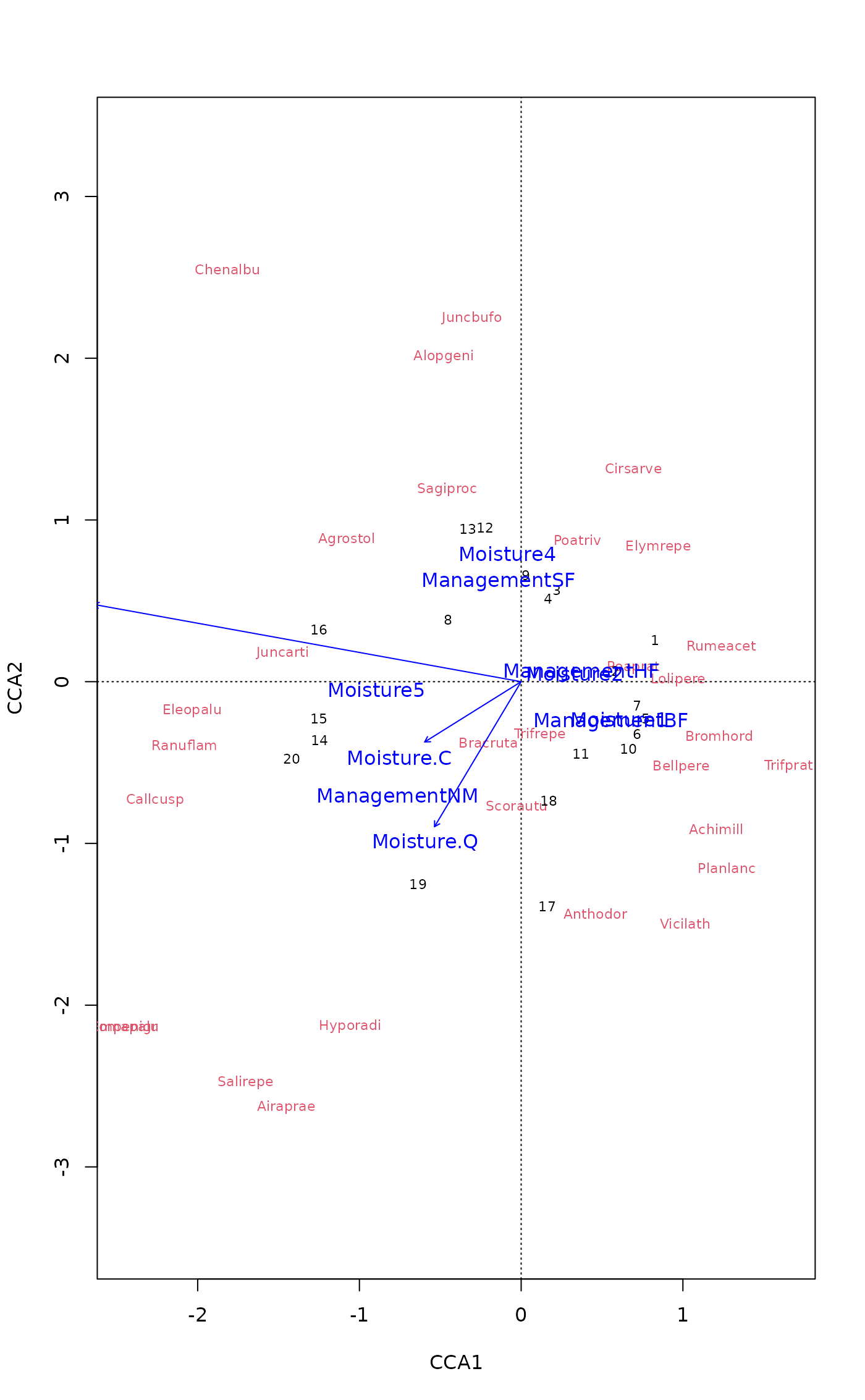
mod <- cca(dune ~ Moisture + Management, dune.env)

## default and modified plot
plot(mod, scaling="sites")

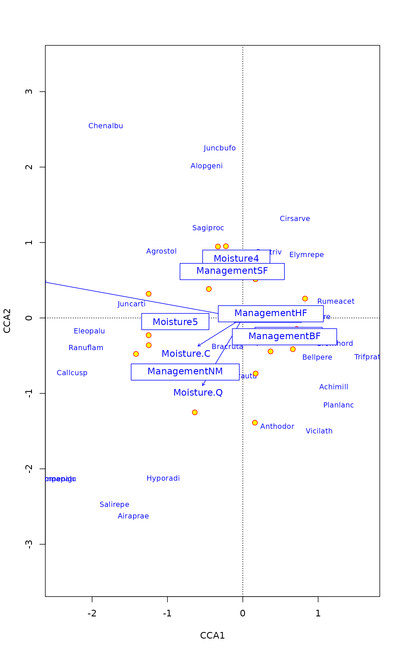
plot(mod, scaling="sites", type = "text",
  sit.par = list(type = "points", pch=21, col="red", bg="yellow", cex=1.2),
  spe.par = list(col="blue", cex=0.8, optimize = TRUE),
  cen.par = list(bg="white"))


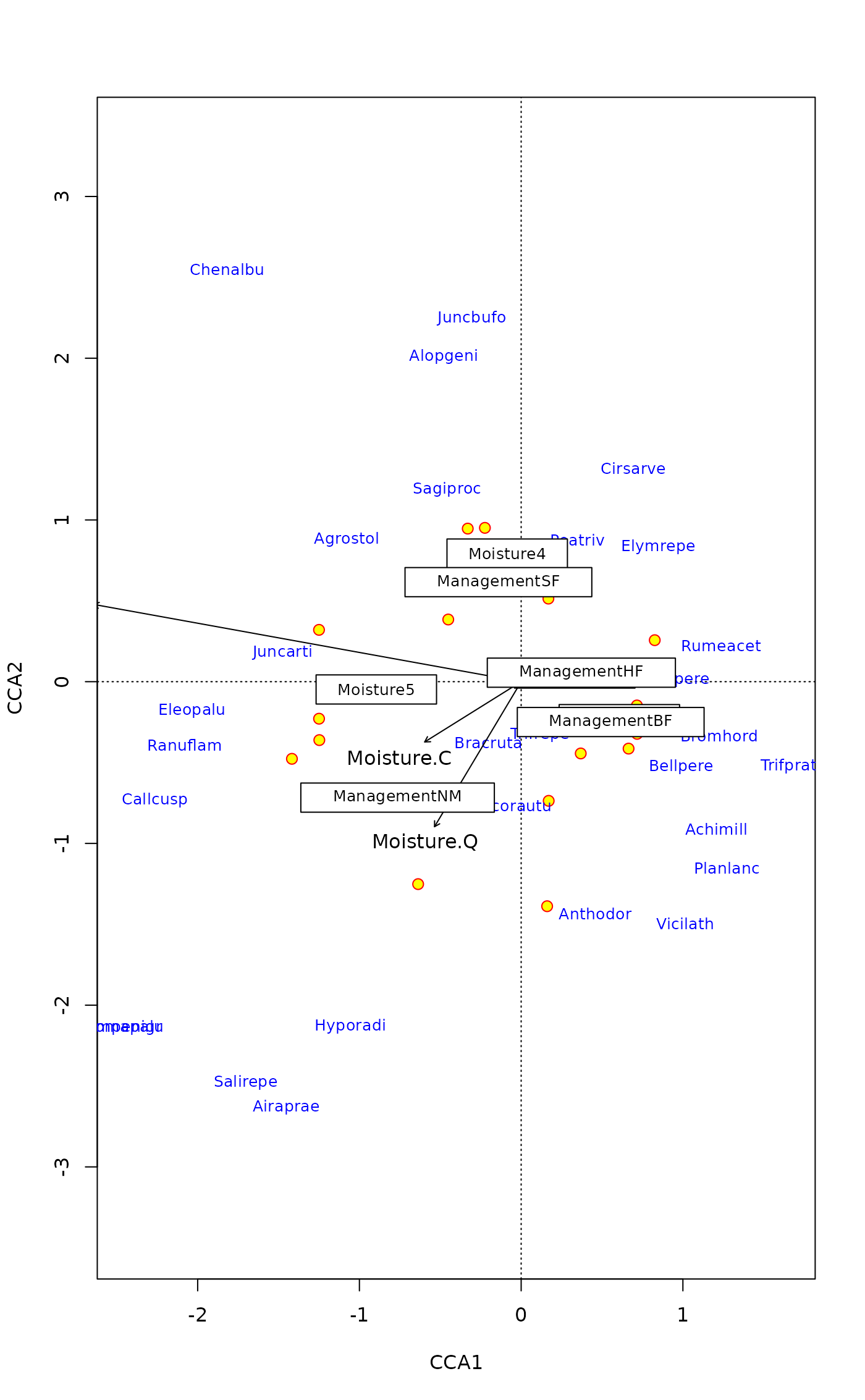
## same with pipe
plot(mod, type="n", scaling="sites") |>
  points("sites", pch=21, col="red", bg = "yellow", cex=1.2) |>
  text("species", col="blue", cex=0.8) |>
  text("biplot") |>
  text("centroids", bg="white")


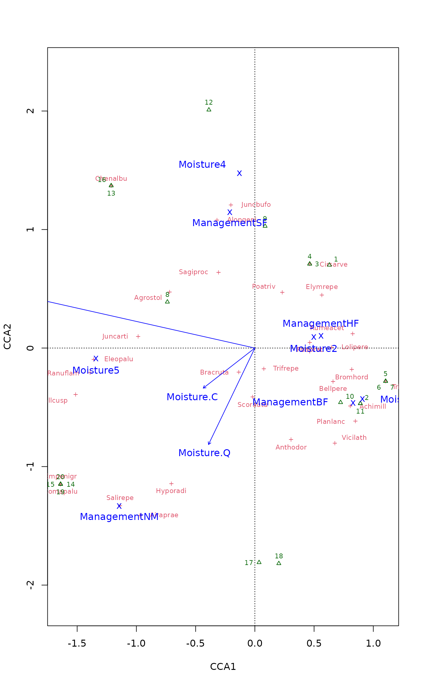
## LC scores & factors mean much overplotting: try optimize=TRUE
plot(mod, display = c("lc","sp","cn"), optimize = TRUE,
   bip.par = list(optimize = FALSE)) # arrows and optimize mix poorly


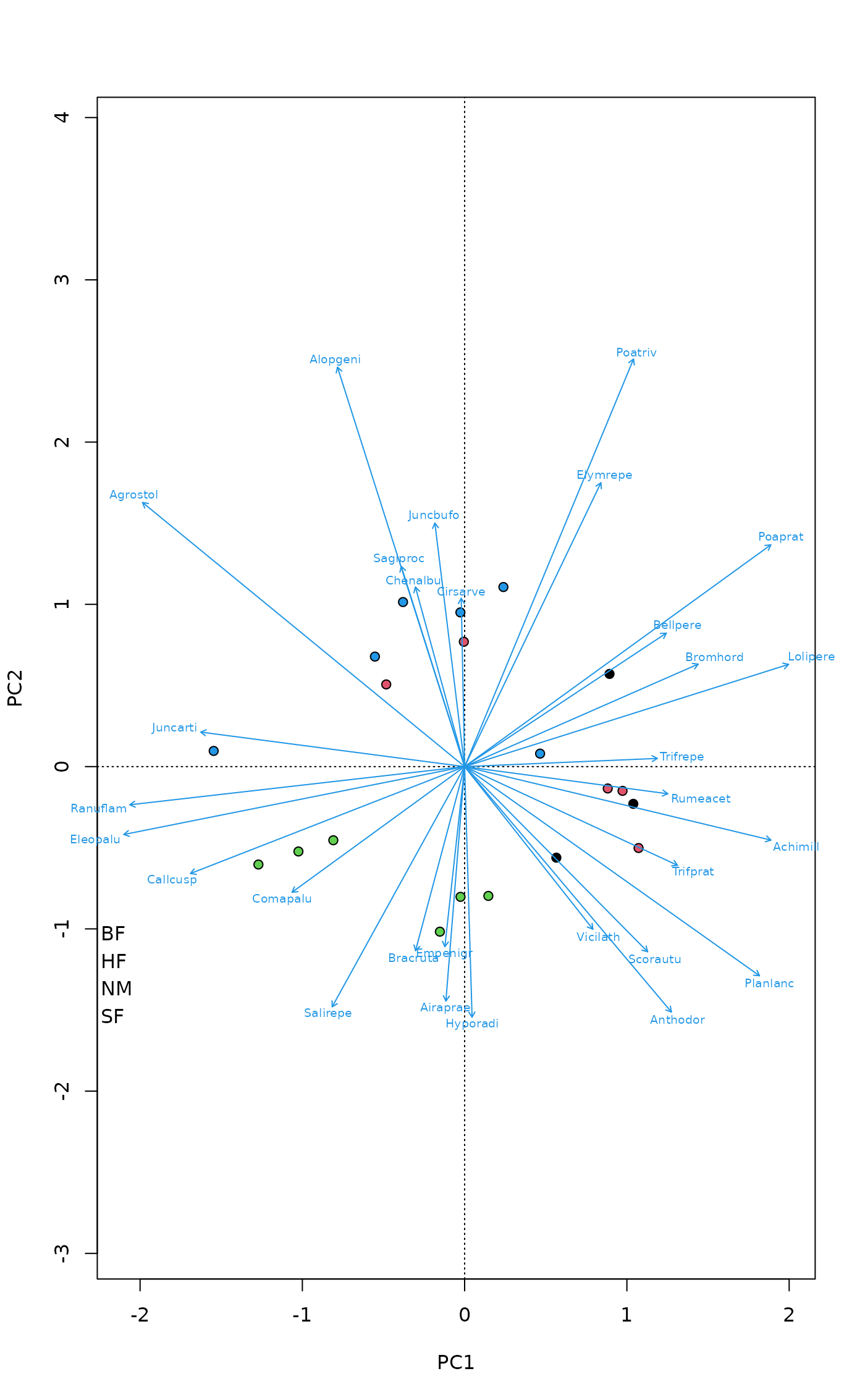
## catch the invisible result and use ordiplot support - the example
## will make a biplot with arrows for species and correlation scaling
pca <- rda(dune)
pl <- plot(pca, type="n", scaling="sites", correlation=TRUE)
with(dune.env, points(pl, "site", pch=21, col=1, bg=Management))
text(pl, "sp", arrow=TRUE, length=0.05, col=4, cex=0.6, xpd=TRUE)
with(dune.env, legend("bottomleft", levels(Management), pch=21,
   pt.bg=1:4, bty="n"))


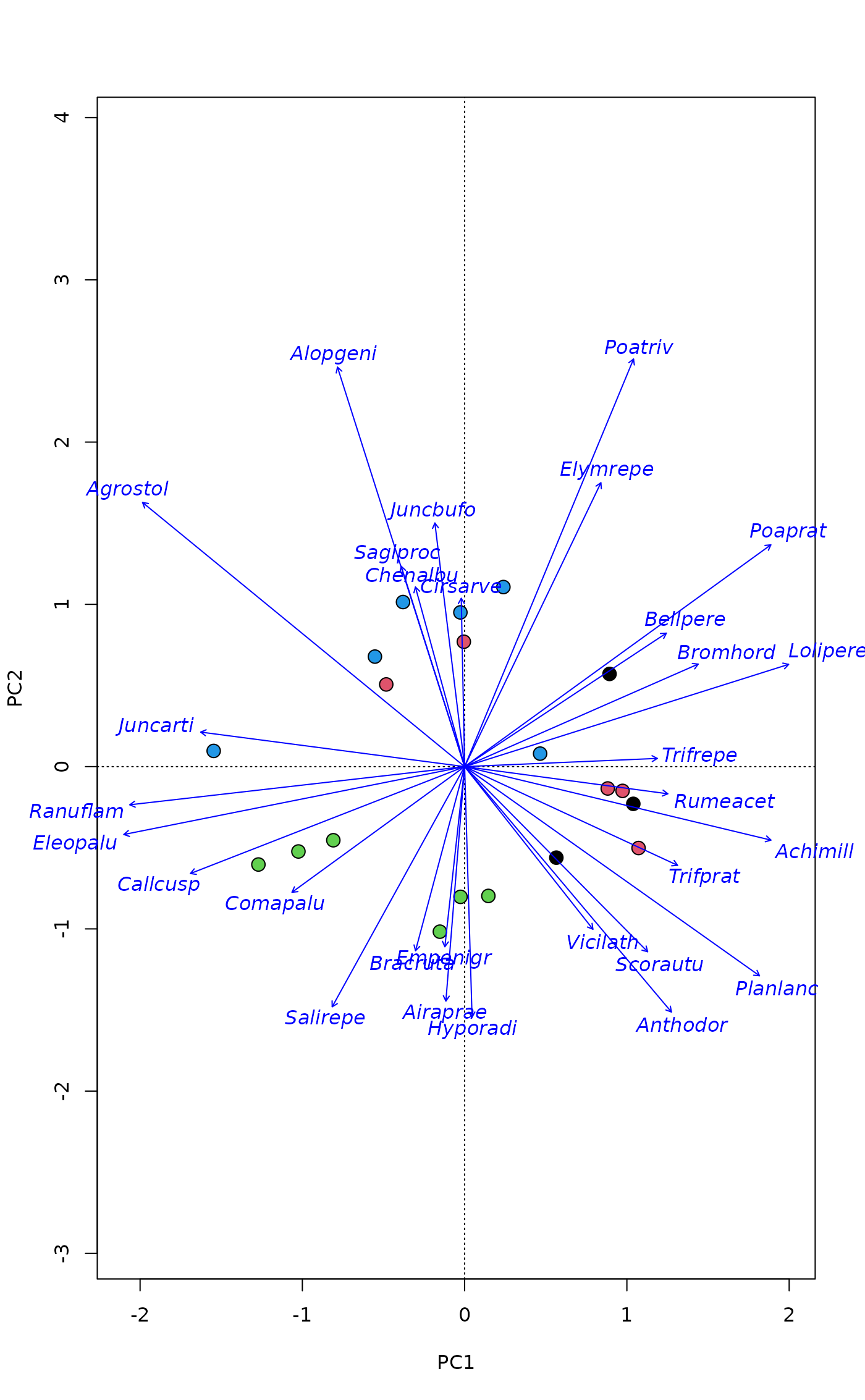
## Pipe
plot(pca, type="n", scaling="sites", correlation=TRUE) |>
    points("sites", pch=21, col = 1, cex=1.5, bg = dune.env$Management) |>
    text("species", col = "blue", arrows = TRUE, xpd = TRUE, font = 3)


## Scaling can be numeric or more user-friendly names
## e.g. Hill's scaling for (C)CA
scrs <- scores(mod, scaling = "sites", hill = TRUE)
## or correlation-based scores in PCA/RDA
scrs <- scores(rda(dune ~ A1 + Moisture + Management, dune.env),
               scaling = "sites", correlation = TRUE)