Fit Fisher's Logseries and Preston's Lognormal Model to Abundance Data

Function fisherfit fits Fisher's logseries to abundance data. Function prestonfit groups species frequencies into doubling octave classes and fits Preston's lognormal model, and function prestondistr fits the truncated lognormal model without pooling the data into octaves.

Usage

fisherfit(x, ...)
prestonfit(x, tiesplit = TRUE, ...)
prestondistr(x, truncate = -1, ...)
# S3 method for prestonfit
plot(x, xlab = "Frequency", ylab = "Species", bar.col = "skyblue", 
    line.col = "red", lwd = 2, ...)
# S3 method for prestonfit
lines(x, line.col = "red", lwd = 2, ...)
veiledspec(x, ...)
as.fisher(x, ...)
# S3 method for fisher
plot(x, xlab = "Frequency", ylab = "Species", bar.col = "skyblue",
             kind = c("bar", "hiplot", "points", "lines"), add = FALSE, ...)
as.preston(x, tiesplit = TRUE, ...)
# S3 method for preston
plot(x, xlab = "Frequency", ylab = "Species", bar.col = "skyblue", ...)
# S3 method for preston
lines(x, xadjust = 0.5, ...)

Arguments

x

Community data vector for fitting functions or their result object for plot functions.

tiesplit

Split frequencies \(1, 2, 4, 8\) etc between adjacent octaves.

truncate

Truncation point for log-Normal model, in log2 units. Default value \(-1\) corresponds to the left border of zero Octave. The choice strongly influences the fitting results.

xlab, ylab

Labels for x and y axes.

bar.col

Colour of data bars.

line.col

Colour of fitted line.

lwd

Width of fitted line.

kind

Kind of plot to drawn: "bar" is similar bar plot as in plot.fisherfit, "hiplot" draws vertical lines as with plot(..., type="h"), and "points" and "lines" are obvious.

add

Add to an existing plot.

xadjust

Adjustment of horizontal positions in octaves.

...

Other parameters passed to functions. Ignored in prestonfit and tiesplit passed to as.preston in prestondistr.

Details

In Fisher's logarithmic series the expected number of species \(f\) with \(n\) observed individuals is \(f_n = \alpha x^n / n\) (Fisher et al. 1943). The estimation is possible only for genuine counts of individuals. The parameter \(\alpha\) is used as a diversity index which can be estimated with a separate function fisher.alpha. The parameter \(x\) is taken as a nuisance parameter which is not estimated separately but taken to be \(n/(n+\alpha)\). Helper function as.fisher transforms abundance data into Fisher frequency table. Diversity will be given as NA for communities with one (or zero) species: there is no reliable way of estimating their diversity, even if the equations will return a bogus numeric value in some cases.

Preston (1948) was not satisfied with Fisher's model which seemed to imply infinite species richness, and postulated that rare species is a diminishing class and most species are in the middle of frequency scale. This was achieved by collapsing higher frequency classes into wider and wider “octaves” of doubling class limits: 1, 2, 3--4, 5--8, 9--16 etc. occurrences. It seems that Preston regarded frequencies 1, 2, 4, etc.. as “tied” between octaves (Williamson & Gaston 2005). This means that only half of the species with frequency 1 are shown in the lowest octave, and the rest are transferred to the second octave. Half of the species from the second octave are transferred to the higher one as well, but this is usually not as large a number of species. This practise makes data look more lognormal by reducing the usually high lowest octaves. This can be achieved by setting argument tiesplit = TRUE. With tiesplit = FALSE the frequencies are not split, but all ones are in the lowest octave, all twos in the second, etc. Williamson & Gaston (2005) discuss alternative definitions in detail, and they should be consulted for a critical review of log-Normal model.

Any logseries data will look like lognormal when plotted in Preston's way. The expected frequency \(f\) at abundance octave \(o\) is defined by \(f_o = S_0 \exp(-(\log_2(o) - \mu)^2/2/\sigma^2)\), where \(\mu\) is the location of the mode and \(\sigma\) the width, both in \(\log_2\) scale, and \(S_0\) is the expected number of species at mode. The lognormal model is usually truncated on the left so that some rare species are not observed. Function prestonfit fits the truncated lognormal model as a second degree log-polynomial to the octave pooled data using Poisson (when tiesplit = FALSE) or quasi-Poisson (when tiesplit = TRUE) error. Function prestondistr fits left-truncated Normal distribution to \(\log_2\) transformed non-pooled observations with direct maximization of log-likelihood. Function prestondistr is modelled after function fitdistr which can be used for alternative distribution models.

The functions have common print, plot and lines methods. The lines function adds the fitted curve to the octave range with line segments showing the location of the mode and the width (sd) of the response. Function as.preston transforms abundance data to octaves. Argument tiesplit will not influence the fit in prestondistr, but it will influence the barplot of the octaves.

The total extrapolated richness from a fitted Preston model can be found with function veiledspec. The function accepts results both from prestonfit and from prestondistr. If veiledspec is called with a species count vector, it will internally use prestonfit. Function specpool provides alternative ways of estimating the number of unseen species. In fact, Preston's lognormal model seems to be truncated at both ends, and this may be the main reason why its result differ from lognormal models fitted in Rank--Abundance diagrams with functions rad.lognormal.

Value

The function prestonfit returns an object with fitted

coefficients, and with observed (freq) and fitted (fitted) frequencies, and a string describing the fitting

method. Function prestondistr omits the entry

fitted. The function fisherfit returns the result of

nlm, where item estimate is \(\alpha\). The result object is amended with the nuisance parameter and item

fisher for the observed data from as.fisher

References

Fisher, R.A., Corbet, A.S. & Williams, C.B. (1943). The relation between the number of species and the number of individuals in a random sample of animal population. Journal of Animal Ecology 12: 42--58.

Preston, F.W. (1948) The commonness and rarity of species. Ecology 29, 254--283.

Williamson, M. & Gaston, K.J. (2005). The lognormal distribution is not an appropriate null hypothesis for the species--abundance distribution. Journal of Animal Ecology 74, 409--422.

Author

Bob O'Hara and Jari Oksanen.

See also

diversity, fisher.alpha, radfit, specpool. Function fitdistr of MASS package was used as the model for prestondistr. Function density can be used for smoothed non-parametric estimation of responses, and qqplot is an alternative, traditional and more effective way of studying concordance of observed abundances to any distribution model.

Examples

data(BCI)
mod <- fisherfit(BCI[5,])
mod
#> 
#> Fisher log series model
#> No. of species: 101 
#> Fisher alpha:   37.96423 
#> 
# prestonfit seems to need large samples
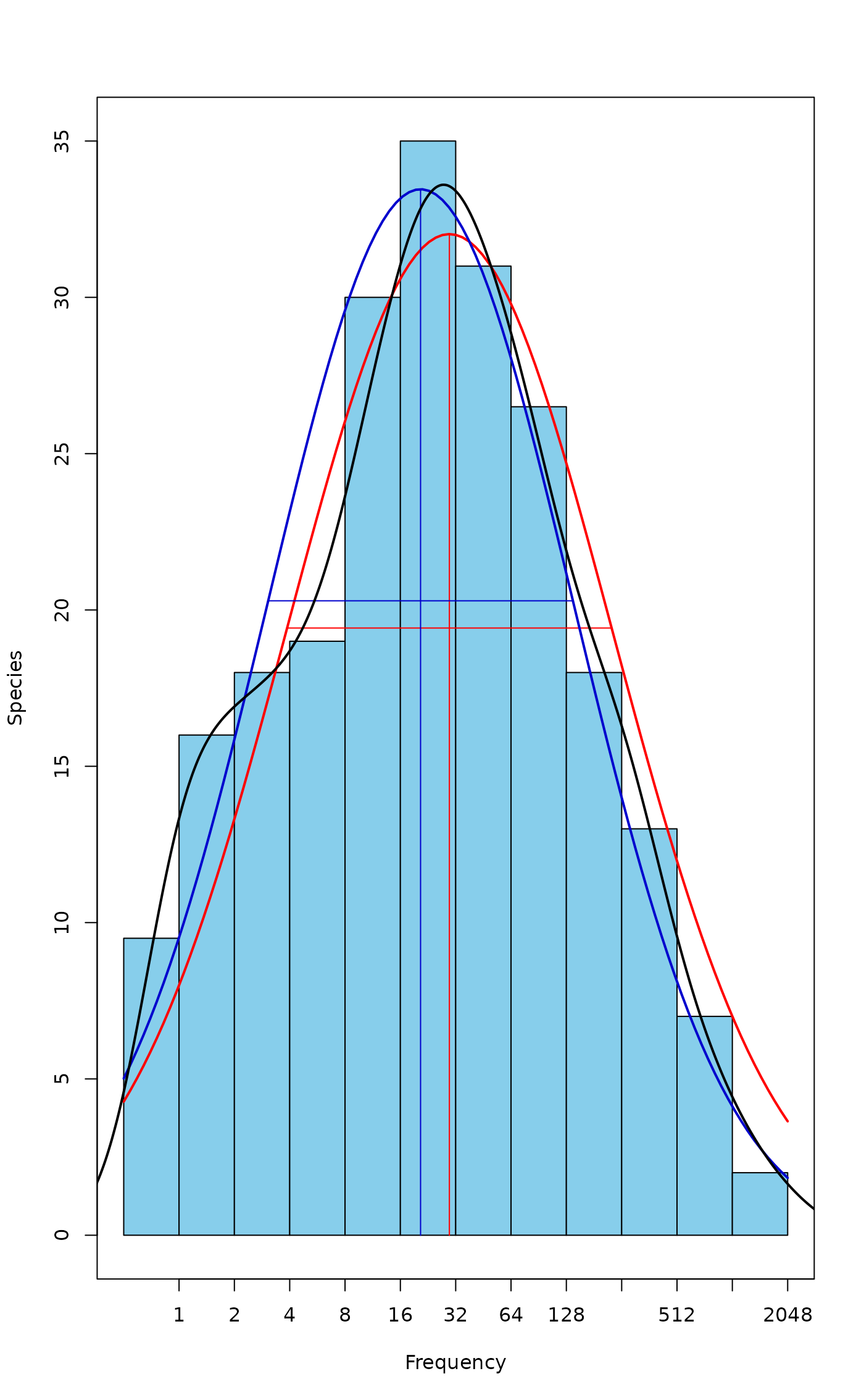
mod.oct <- prestonfit(colSums(BCI))
mod.ll <- prestondistr(colSums(BCI))
mod.oct
#> 
#> Preston lognormal model
#> Method: Quasi-Poisson fit to octaves 
#> No. of species: 225 
#> 
#>      mode     width        S0 
#>  4.885798  2.932690 32.022923 
#> 
#> Frequencies by Octave
#>                 0        1        2      3        4        5        6        7
#> Observed 9.500000 16.00000 18.00000 19.000 30.00000 35.00000 31.00000 26.50000
#> Fitted   7.994154 13.31175 19.73342 26.042 30.59502 31.99865 29.79321 24.69491
#>                 8        9       10     11
#> Observed 18.00000 13.00000 7.000000 2.0000
#> Fitted   18.22226 11.97021 7.000122 3.6443
#> 
mod.ll
#> 
#> Preston lognormal model
#> Method: maximized likelihood to log2 abundances 
#> No. of species: 225 
#> 
#>      mode     width        S0 
#>  4.365002  2.753531 33.458185 
#> 
#> Frequencies by Octave
#>                0        1        2        3        4        5        6        7
#> Observed 9.50000 16.00000 18.00000 19.00000 30.00000 35.00000 31.00000 26.50000
#> Fitted   9.52392 15.85637 23.13724 29.58961 33.16552 32.58022 28.05054 21.16645
#>                 8         9       10      11
#> Observed 18.00000 13.000000 7.000000 2.00000
#> Fitted   13.99829  8.113746 4.121808 1.83516
#> 
plot(mod.oct)  
lines(mod.ll, line.col="blue3") # Different
## Smoothed density
den <- density(log2(colSums(BCI)))
lines(den$x, ncol(BCI)*den$y, lwd=2) # Fairly similar to mod.oct

## Extrapolated richness
veiledspec(mod.oct)
#> Extrapolated     Observed       Veiled 
#>    235.40577    225.00000     10.40577 
veiledspec(mod.ll)
#> Extrapolated     Observed       Veiled 
#>   230.931018   225.000000     5.931018