Extrapolated Species Richness in a Species Pool

The functions estimate the extrapolated species richness in a species pool, or the number of unobserved species. Function specpool is based on incidences in sample sites, and gives a single estimate for a collection of sample sites (matrix). Function estimateR is based on abundances (counts) on single sample site.

Usage

specpool(x, pool, smallsample = TRUE)
estimateR(x, ...)
specpool2vect(X, index = c("jack1","jack2", "chao", "boot","Species"))
poolaccum(x, permutations = 100, minsize = 3)
estaccumR(x, permutations = 100, parallel = getOption("mc.cores"))
# S3 method for poolaccum
summary(object, display, alpha = 0.05, ...)
# S3 method for poolaccum
plot(x, alpha = 0.05, type = c("l","g"), ...)

Arguments

x: Data frame or matrix with species data or the analysis result for plot function.
pool: A vector giving a classification for pooling the sites in the species data. If missing, all sites are pooled together.
smallsample: Use small sample correction \((N-1)/N\), where \(N\) is the number of sites within the pool.
X, object: A specpool result object.
index: The selected index of extrapolated richness.
permutations: Usually an integer giving the number permutations, but can also be a list of control values for the permutations as returned by the function how, or a permutation matrix where each row gives the permuted indices.
minsize: Smallest number of sampling units reported.
parallel: Number of parallel processes or a predefined socket cluster. With parallel = 1 uses ordinary, non-parallel processing. The parallel processing is done with parallel package.
display: Indices to be displayed.
alpha: Level of quantiles shown. This proportion will be left outside symmetric limits.
type: Type of graph produced in xyplot.
...: Other parameters (not used).

Details

Many species will always remain unseen or undetected in a collection of sample plots. The function uses some popular ways of estimating the number of these unseen species and adding them to the observed species richness (Palmer 1990, Colwell & Coddington 1994).

The incidence-based estimates in specpool use the frequencies of species in a collection of sites. In the following, \(S_P\) is the extrapolated richness in a pool, \(S_0\) is the observed number of species in the collection, \(a_1\) and \(a_2\) are the number of species occurring only in one or only in two sites in the collection, \(p_i\) is the frequency of species \(i\), and \(N\) is the number of sites in the collection. The variants of extrapolated richness in specpool are:

Chao	\(S_P = S_0 + \frac{a_1^2}{2 a_2}\frac{N-1}{N}\)
Chao bias-corrected	\(S_P = S_0 + \frac{a_1(a_1-1)}{2(a_2+1)} \frac{N-1}{N}\)
First order jackknife	\(S_P = S_0 + a_1 \frac{N-1}{N}\)
Second order jackknife	\(S_P = S_0 + a_1 \frac{2N - 3}{N} - a_2 \frac{(N-2)^2}{N (N-1)}\)
Bootstrap	\(S_P = S_0 + \sum_{i=1}^{S_0} (1 - p_i)^N\)

specpool normally uses basic Chao equation, but when there are no doubletons (\(a2=0\)) it switches to bias-corrected version. In that case the Chao equation simplifies to \(S_0 + \frac{1}{2} a_1 (a_1-1) \frac{N-1}{N}\).

The abundance-based estimates in estimateR use counts (numbers of individuals) of species in a single site. If called for a matrix or data frame, the function will give separate estimates for each site. The two variants of extrapolated richness in estimateR are bias-corrected Chao and ACE (O'Hara 2005, Chiu et al. 2014). The Chao estimate is similar as the bias corrected one above, but \(a_i\) refers to the number of species with abundance \(i\) instead of number of sites, and the small-sample correction is not used. The ACE estimate is defined as:

ACE	\(S_P = S_{abund} + \frac{S_{rare}}{C_{ace}}+ \frac{a_1}{C_{ace}} \gamma^2_{ace}\)
where	\(C_{ace} = 1 - \frac{a_1}{N_{rare}}\)
	\(\gamma^2_{ace} = \max \left[ \frac{S_{rare} \sum_{i=1}^{10} i(i-1)a_i}{C_{ace} N_{rare} (N_{rare} - 1)}-1, 0 \right]\)

Here \(a_i\) refers to number of species with abundance \(i\) and \(S_{rare}\) is the number of rare species, \(S_{abund}\) is the number of abundant species, with an arbitrary threshold of abundance 10 for rare species, and \(N_{rare}\) is the number of individuals in rare species.

Functions estimate the standard errors of the estimates. These only concern the number of added species, and assume that there is no variance in the observed richness. The equations of standard errors are too complicated to be reproduced in this help page, but they can be studied in the R source code of the function and are discussed in the vignette that can be read with the browseVignettes("vegan"). The standard error are based on the following sources: Chiu et al. (2014) for the Chao estimates and Smith and van Belle (1984) for the first-order Jackknife and the bootstrap (second-order jackknife is still missing). For the variance estimator of \(S_{ace}\) see O'Hara (2005).

Functions poolaccum and estaccumR are similar to specaccum, but estimate extrapolated richness indices of specpool or estimateR in addition to number of species for random ordering of sampling units. Function specpool uses presence data and estaccumR count data. The functions share summary and plot methods. The summary returns quantile envelopes of permutations corresponding the given level of alpha and standard deviation of permutations for each sample size. NB., these are not based on standard deviations estimated within specpool or estimateR, but they are based on permutations. The plot function shows the mean and envelope of permutations with given alpha for models. The selection of models can be restricted and order changes using the display argument in summary or plot. For configuration of plot command, see xyplot.

Value

Function specpool returns a data frame with entries for observed richness and each of the indices for each class in

pool vector. The utility function specpool2vect maps the pooled values into a vector giving the value of selected

index for each original site. Function estimateR

returns the estimates and their standard errors for each site. Functions poolaccum and estimateR return matrices of permutation results for each richness estimator, the vector of sample sizes and a table of means of permutations for each estimator.

References

Chao, A. (1987). Estimating the population size for capture-recapture data with unequal catchability. Biometrics 43, 783--791.

Chiu, C.H., Wang, Y.T., Walther, B.A. & Chao, A. (2014). Improved nonparametric lower bound of species richness via a modified Good-Turing frequency formula. Biometrics 70, 671--682.

Colwell, R.K. & Coddington, J.A. (1994). Estimating terrestrial biodiversity through extrapolation. Phil. Trans. Roy. Soc. London B 345, 101--118.

O'Hara, R.B. (2005). Species richness estimators: how many species can dance on the head of a pin? J. Anim. Ecol. 74, 375--386.

Palmer, M.W. (1990). The estimation of species richness by extrapolation. Ecology 71, 1195--1198.

Smith, E.P & van Belle, G. (1984). Nonparametric estimation of species richness. Biometrics 40, 119--129.

Author

Bob O'Hara (estimateR) and Jari Oksanen.

Note

The functions are based on assumption that there is a species pool: The community is closed so that there is a fixed pool size \(S_P\). In general, the functions give only the lower limit of species richness: the real richness is \(S >= S_P\), and there is a consistent bias in the estimates. Even the bias-correction in Chao only reduces the bias, but does not remove it completely (Chiu et al. 2014).

Optional small sample correction was added to specpool in vegan 2.2-0. It was not used in the older literature (Chao 1987), but it is recommended recently (Chiu et al. 2014).

Examples

data(dune)
data(dune.env)
pool <- with(dune.env, specpool(dune, Management))
pool
#>    Species     chao   chao.se    jack1 jack1.se    jack2     boot  boot.se n
#> BF      16 17.19048 1.5895675 19.33333 2.211083 19.83333 17.74074 1.646379 3
#> HF      21 21.51429 0.9511693 23.40000 1.876166 22.05000 22.56864 1.821518 5
#> NM      21 22.87500 2.1582871 26.00000 3.291403 25.73333 23.77696 2.300982 6
#> SF      21 29.88889 8.6447967 27.66667 3.496029 31.40000 23.99496 1.850288 6
op <- par(mfrow=c(1,2))
boxplot(specnumber(dune) ~ Management, data = dune.env,
        col = "hotpink", border = "cyan3")
boxplot(specnumber(dune)/specpool2vect(pool) ~ Management,
        data = dune.env, col = "hotpink", border = "cyan3")

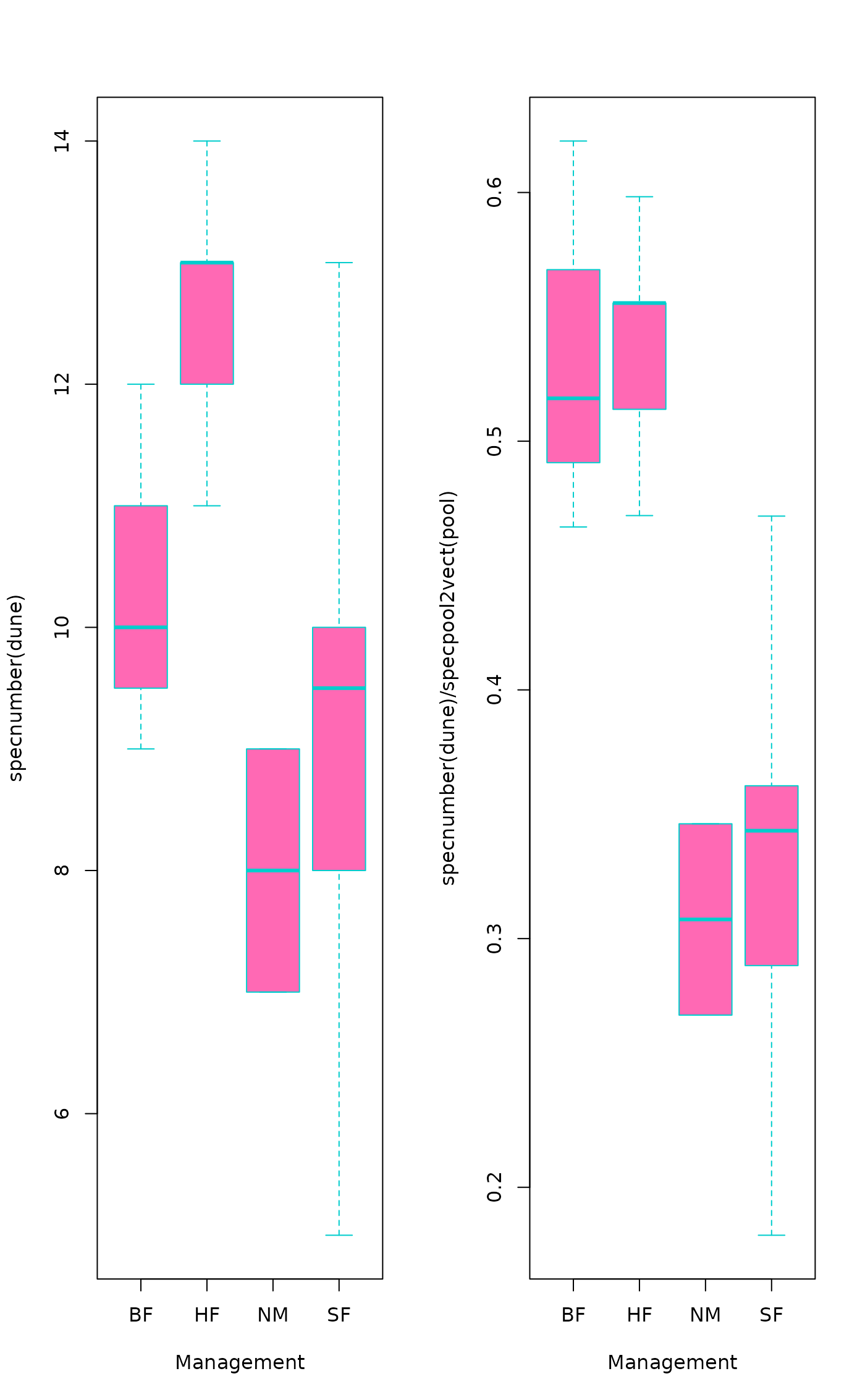par(op)
data(BCI)
## Accumulation model
pool <- poolaccum(BCI)
summary(pool, display = "chao")
#> $chao
#>        N     Chao     2.5%    97.5%   Std.Dev
#>  [1,]  3 162.3374 142.5272 186.2227 11.217082
#>  [2,]  4 176.1243 156.4704 206.3243 12.158304
#>  [3,]  5 183.8507 162.9868 209.2821 12.488675
#>  [4,]  6 188.9018 165.6732 214.2779 12.888148
#>  [5,]  7 193.8679 175.8712 216.1384 11.602711
#>  [6,]  8 199.0315 180.2949 227.8918 12.604562
#>  [7,]  9 202.0946 183.3317 228.8381 11.958432
#>  [8,] 10 204.9843 185.3556 227.5898 12.637762
#>  [9,] 11 206.6160 186.7205 234.5167 11.679759
#> [10,] 12 209.1286 189.2824 232.6359 12.351073
#> [11,] 13 211.3655 191.7918 232.0423 11.991967
#> [12,] 14 212.8128 195.8592 239.3318 11.537817
#> [13,] 15 215.5275 198.2739 239.7978 11.422201
#> [14,] 16 218.7094 198.3891 243.3826 12.165145
#> [15,] 17 221.6814 197.6029 256.5328 14.464302
#> [16,] 18 222.7418 201.4964 257.9494 13.227892
#> [17,] 19 224.8619 206.6236 251.9979 13.165360
#> [18,] 20 226.3324 210.2832 249.5616 12.858116
#> [19,] 21 228.4284 210.9920 257.9636 13.784663
#> [20,] 22 228.8425 211.1903 254.3500 11.629250
#> [21,] 23 230.6429 214.1737 251.1681 10.510649
#> [22,] 24 231.9109 213.0874 252.7553 10.925851
#> [23,] 25 232.9972 214.3610 258.4917 11.207306
#> [24,] 26 233.8067 216.9697 263.2733 11.546339
#> [25,] 27 235.6347 217.3831 266.9230 12.800245
#> [26,] 28 235.8942 218.6913 261.4115 11.761873
#> [27,] 29 235.9612 218.6591 258.5682 11.133700
#> [28,] 30 236.6706 219.4315 259.9315 10.291499
#> [29,] 31 236.8530 220.2338 259.2903  9.810390
#> [30,] 32 237.6018 221.4868 262.0864 10.195825
#> [31,] 33 237.4291 222.2990 256.2778  9.227891
#> [32,] 34 237.6712 222.7844 258.2268  8.979536
#> [33,] 35 237.7856 222.2750 257.2540  8.537867
#> [34,] 36 238.4325 223.6473 255.5610  8.566487
#> [35,] 37 238.1834 224.9892 253.5811  7.776992
#> [36,] 38 238.4685 225.2802 254.0155  7.626532
#> [37,] 39 238.2082 226.0390 252.7975  7.642443
#> [38,] 40 238.7991 227.1971 254.1619  7.155802
#> [39,] 41 239.2246 227.3368 258.5178  7.926574
#> [40,] 42 238.4935 228.5195 256.2137  7.287824
#> [41,] 43 238.3856 227.8327 255.8470  7.300153
#> [42,] 44 238.0092 228.5279 252.9488  6.520961
#> [43,] 45 238.1537 228.7980 253.3757  6.443894
#> [44,] 46 238.0532 230.5990 250.9539  5.466587
#> [45,] 47 237.7542 231.3089 251.0192  4.821564
#> [46,] 48 237.2842 231.9015 248.6399  4.038862
#> [47,] 49 236.8407 233.3115 245.4082  2.803888
#> [48,] 50 236.3732 236.3732 236.3732  0.000000
#> 
#> attr(,"class")
#> [1] "summary.poolaccum"
plot(pool)

## Quantitative model
estimateR(BCI[1:5,])
#>                   1          2          3          4          5
#> S.obs     93.000000  84.000000  90.000000  94.000000 101.000000
#> S.chao1  117.473684 117.214286 141.230769 111.550000 136.000000
#> se.chao1  11.583785  15.918953  23.001405   8.919663  15.467344
#> S.ACE    122.848959 117.317307 134.669844 118.729941 137.114088
#> se.ACE     5.736054   5.571998   6.191618   5.367571   5.848474