Rank – Abundance or Dominance / Diversity Models

Functions construct rank – abundance or dominance / diversity or Whittaker plots and fit brokenstick, preemption, log-Normal, Zipf and Zipf-Mandelbrot models of species abundance.

Usage

# Default S3 method
radfit(x, ...)
rad.null(x, family=poisson, ...)
rad.preempt(x, family = poisson, ...)
rad.lognormal(x, family = poisson, ...)
rad.zipf(x, family = poisson, ...)
rad.zipfbrot(x, family = poisson, ...)
# S3 method for class 'radline'
predict(object, newdata, total, ...)
# S3 method for class 'radfit'
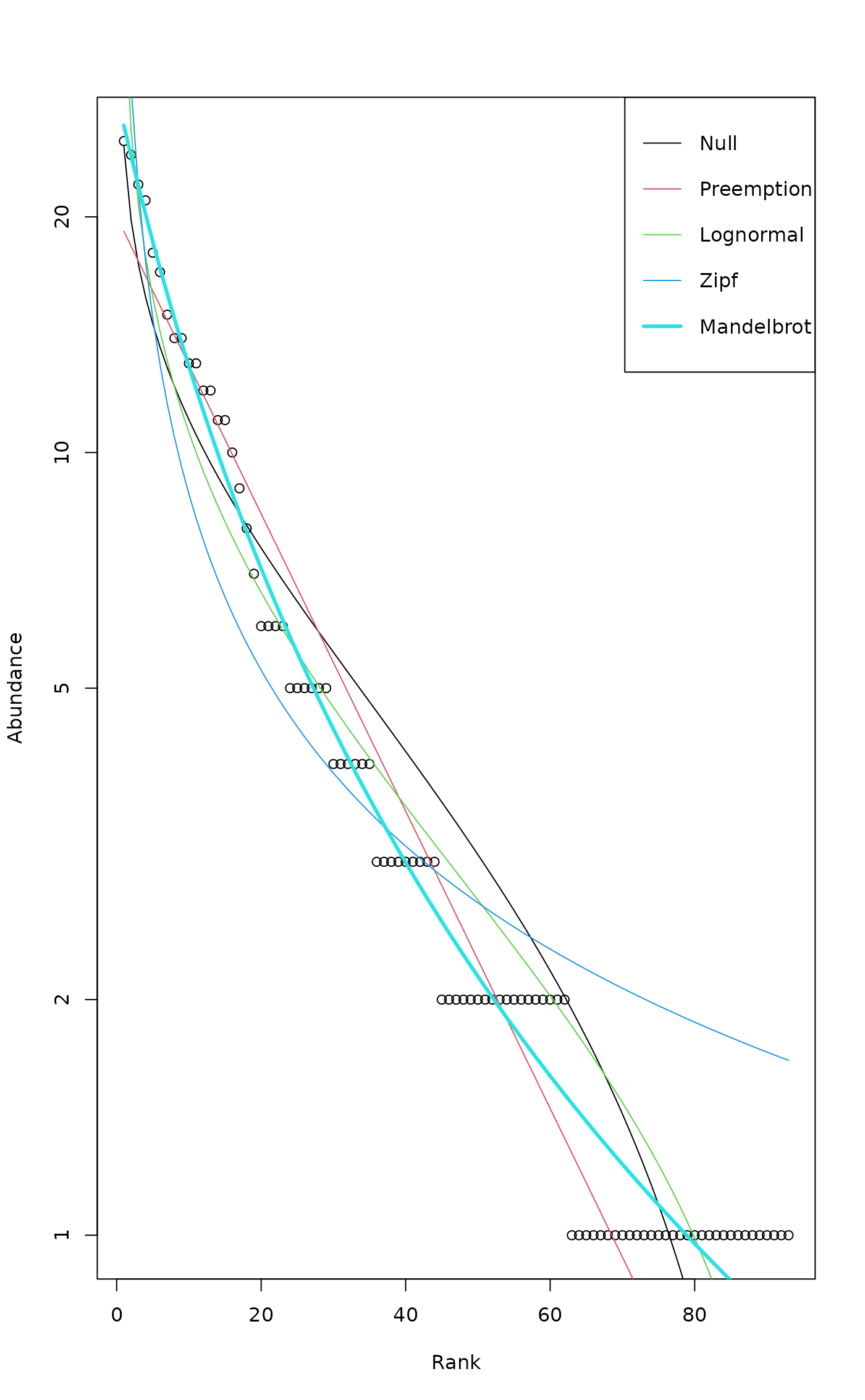
plot(x, BIC = FALSE, legend = TRUE, ...)
# S3 method for class 'radfit.frame'
plot(x, order.by, BIC = FALSE, model, legend = TRUE,
     as.table = TRUE, ...)
# S3 method for class 'radline'
plot(x, xlab = "Rank", ylab = "Abundance", type = "b", ...)
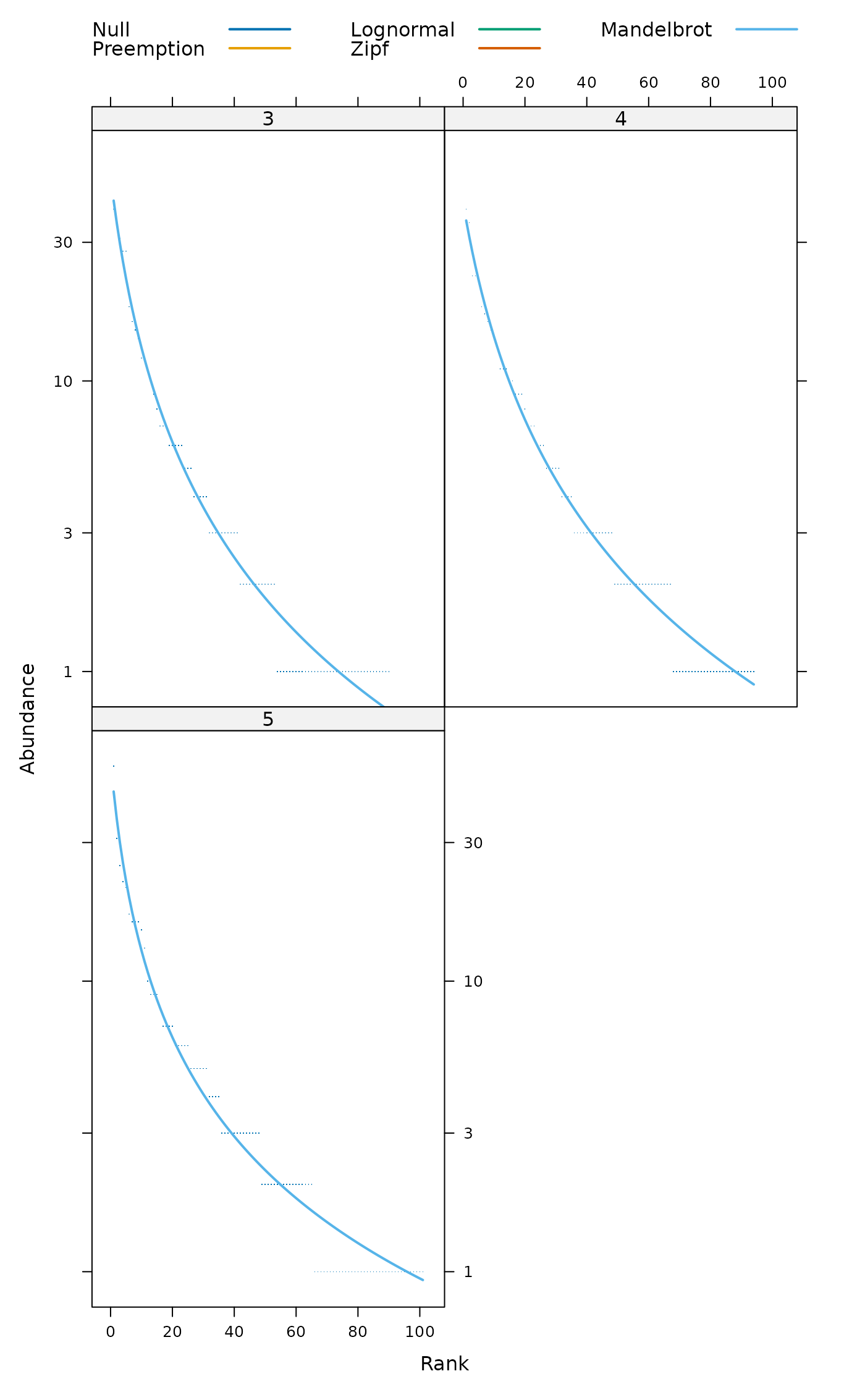
radlattice(x, BIC = FALSE, ...)
# S3 method for class 'radfit'
lines(x, ...)
# S3 method for class 'radfit'
points(x, ...)
as.rad(x)
# S3 method for class 'rad'
plot(x, xlab = "Rank", ylab = "Abundance", log = "y", ...)

Arguments

x: Data frame, matrix or a vector giving species abundances, or an object to be plotted.
family: Error distribution (passed to glm). All alternatives accepting link = "log" in family can be used, although not all make sense.
object: A fitted result object.
newdata: Ranks used for ordinations. All models can interpolate to non-integer “ranks” (although this may be approximate), but extrapolation may fail
total: The new total used for predicting abundance. Observed total count is used if this is omitted.
order.by: A vector used for ordering sites in plots.
BIC: Use Bayesian Information Criterion, BIC, instead of Akaike's AIC. The penalty in BIC is \(k = \log(S)\) where \(S\) is the number of species, whereas AIC uses \(k = 2\).
model: Show only the specified model. If missing, AIC is used to select the model. The model names (which can be abbreviated) are Null, Preemption, Lognormal, Zipf, Mandelbrot.
legend: Add legend of line colours.
as.table: Arrange panels starting from upper left corner (passed to xyplot).
xlab,ylab: Labels for x and y axes.
type: Type of the plot, "b" for plotting both observed points and fitted lines, "p" for only points, "l" for only fitted lines, and "n" for only setting the frame.
log: Use logarithmic scale for given axis. The default log = "y" gives the traditional plot of community ecology where the preemption model is a straight line, and with log = "xy" Zipf model is a straight line. With log = "" both axes are in the original arithmetic scale.
...: Other parameters to functions.

Details

Rank–Abundance Dominance (RAD) or Dominance/Diversity plots (Whittaker 1965) display logarithmic species abundances against species rank order. These plots are supposed to be effective in analysing types of abundance distributions in communities. These functions fit some of the most popular models mainly following Wilson (1991).

Functions rad.null, rad.preempt, rad.lognormal, rad.zipf and zipfbrot fit the individual models (described below) for a single vector (row of data frame), and function radfit fits all models. The argument of the function radfit can be either a vector for a single community or a data frame where each row represents a distinct community.

Function rad.null fits a brokenstick model where the expected abundance of species at rank \(r\) is \(a_r = (J/S) \sum_{x=r}^S (1/x)\) (Pielou 1975), where \(J\) is the total number of individuals (site total) and \(S\) is the total number of species in the community. This gives a Null model where the individuals are randomly distributed among observed species, and there are no fitted parameters. Function rad.preempt fits the niche preemption model, a.k.a. geometric series or Motomura model, where the expected abundance \(a\) of species at rank \(r\) is \(a_r = J \alpha (1 - \alpha)^{r-1}\). The only estimated parameter is the preemption coefficient \(\alpha\) which gives the decay rate of abundance per rank. The niche preemption model is a straight line in a RAD plot. Function rad.lognormal fits a log-Normal model which assumes that the logarithmic abundances are distributed Normally, or \(a_r = \exp( \log \mu + \log \sigma N)\), where \(N\) is a Normal deviate. Function rad.zipf fits the Zipf model \(a_r = J p_1 r^\gamma\) where \(p_1\) is the fitted proportion of the most abundant species, and \(\gamma\) is a decay coefficient. The Zipf–Mandelbrot model (rad.zipfbrot) adds one parameter: \(a_r = J c (r + \beta)^\gamma\) after which \(p_1\) of the Zipf model changes into a meaningless scaling constant \(c\).

Log-Normal and Zipf models are generalized linear models (glm) with logarithmic link function. Zipf–Mandelbrot adds one nonlinear parameter to the Zipf model, and is fitted using nlm for the nonlinear parameter and estimating other parameters and log-Likelihood with glm. Preemption model is fitted as a purely nonlinear model. There are no estimated parameters in the Null model.

The default family is poisson which is appropriate only for genuine counts (integers), but other families that accept link = "log" can be used. Families Gamma or gaussian may be appropriate for abundance data, such as cover. The best model is selected by AIC. Therefore ‘quasi’ families such as quasipoisson cannot be used: they do not have AIC nor log-Likelihood needed in non-linear models.

All these functions have their own plot functions. When radfit was applied for a data frame, plot uses Lattice graphics, and other plot functions use ordinary graphics. The ordinary graphics functions return invisibly an ordiplot object for observed points, and function identify.ordiplot can be used to label selected species. Alternatively, radlattice uses Lattice graphics to display each radfit model of a single site in a separate panel together with their AIC or BIC values.

Function as.rad is a base function to construct ordered RAD data. Its plot is used by other RAD plot functions which pass extra arguments (such as xlab and log) to this function. The function returns an ordered vector of taxa occurring in a site, and a corresponding attribute "index" of included taxa.

Value

Functions rad.null, rad.preempt, rad.lognormal, zipf and zipfbrot fit each a single RAD model to a single site. The result object has class "radline" and inherits from glm, and can be handled by some (but not all) glm methods.

Function radfit fits all models either to a single site or to all rows of a data frame or a matrix. When fitted to a single site, the function returns an object of class "radfit" with items y (observed values), family, and models which is a list of fitted "radline" models. When applied for a data frame or matrix, radfit function returns an object of class "radfit.frame" which is a list of "radfit" objects, each item names by the corresponding row name.

All result objects ("radline", "radfit", "radfit.frame") can be accessed with same method functions. The following methods are available: AIC, coef, deviance, logLik. In addition the fit results can be accessed with fitted, predict and residuals (inheriting from residuals.glm). The graphical functions were discussed above in Details.

References

Pielou, E.C. (1975) Ecological Diversity. Wiley & Sons.

Preston, F.W. (1948) The commonness and rarity of species. Ecology 29, 254–283.

Whittaker, R. H. (1965) Dominance and diversity in plant communities. Science 147, 250–260.

Wilson, J. B. (1991) Methods for fitting dominance/diversity curves. Journal of Vegetation Science 2, 35–46.

Author

Jari Oksanen

Note

The RAD models are usually fitted for proportions instead of original abundances. However, nothing in these models seems to require division of abundances by site totals, and original observations are used in these functions. If you wish to use proportions, you must standardize your data by site totals, e.g. with decostand and use appropriate family such as Gamma.

The lognormal model is fitted in a standard way, but I do think this is not quite correct – at least it is not equivalent to fitting Normal density to log abundances like originally suggested (Preston 1948).

Some models may fail. In particular, estimation of the Zipf-Mandelbrot model is difficult. If the fitting fails, NA is returned.

Wilson (1991) defined preemption model as \(a_r = J p_1 (1 - \alpha)^{r-1}\), where \(p_1\) is the fitted proportion of the first species. However, parameter \(p_1\) is completely defined by \(\alpha\) since the fitted proportions must add to one, and therefore I handle preemption as a one-parameter model.

Veiled log-Normal model was included in earlier releases of this function, but it was removed because it was flawed: an implicit veil line also appears in the ordinary log-Normal. The latest release version with rad.veil was 1.6-10.

Examples

data(BCI)
mod <- rad.lognormal(BCI[5,])
mod
#> 
#> RAD model: Log-Normal 
#> Family: poisson 
#> No. of species:  101 
#> Total abundance: 505 
#> 
#>     log.mu  log.sigma   Deviance        AIC        BIC 
#>   0.951926   1.165929  17.077549 317.656487 322.886728 
plot(mod)

mod <- radfit(BCI[1,])
## Standard plot overlaid for all models
## Preemption model is a line
plot(mod)

## log for both axes: Zipf model is a line
plot(mod, log = "xy")

## Lattice graphics separately for each model
radlattice(mod)

# Take a subset of BCI to save time and nerves
mod <- radfit(BCI[3:5,])
mod
#> 
#> Deviance for RAD models:
#> 
#>                  3       4      5
#> Null       86.1127 49.8111 80.855
#> Preemption 58.9295 39.7817 76.311
#> Lognormal  29.2719 16.6588 17.078
#> Zipf       50.1262 47.9108 30.936
#> Mandelbrot  5.7342  5.5665 10.573
plot(mod, pch=".")