Multivariate homogeneity of groups dispersions (variances)
betadisper.RdImplements Marti Anderson's PERMDISP2 procedure for the analysis of
multivariate homogeneity of group dispersions (variances).
betadisper is a multivariate analogue of Levene's test for
homogeneity of variances. Non-euclidean distances between objects and
group centres (centroids or medians) are handled by reducing the
original distances to principal coordinates. This procedure has
latterly been used as a means of assessing beta diversity. There are
anova, scores, plot and boxplot methods.
TukeyHSD.betadisper creates a set of confidence intervals on
the differences between the mean distance-to-centroid of the levels of
the grouping factor with the specified family-wise probability of
coverage. The intervals are based on the Studentized range statistic,
Tukey's 'Honest Significant Difference' method.
Usage
betadisper(d, group, type = c("median","centroid"), bias.adjust = FALSE,
       sqrt.dist = FALSE, add = FALSE)

# S3 method for class 'betadisper'
anova(object, ...)

# S3 method for class 'betadisper'
scores(x, display = c("sites", "centroids"),
       choices = c(1,2), ...)

# S3 method for class 'betadisper'
eigenvals(x, ...)

# S3 method for class 'betadisper'
plot(x, axes = c(1,2), cex = 0.7,
     pch = seq_len(ng), col = NULL, lty = "solid", lwd = 1, hull = TRUE,
     ellipse = FALSE, conf,
     segments = TRUE, seg.col = "grey", seg.lty = lty, seg.lwd = lwd,
     label = TRUE, label.cex = 1,
     ylab, xlab, main, sub, ...)

# S3 method for class 'betadisper'
boxplot(x, ylab = "Distance to centroid", ...)

# S3 method for class 'betadisper'
TukeyHSD(x, which = "group", ordered = FALSE,
         conf.level = 0.95, ...)

# S3 method for class 'betadisper'
print(x, digits = max(3, getOption("digits") - 3),
                           neigen = 8, ...)

betadistances(x, ...)
Arguments
- d
a distance structure such as that returned by
dist,betadiverorvegdist.- group
vector describing the group structure, usually a factor or an object that can be coerced to a factor using
as.factor. Can consist of a factor with a single level (i.e., one group).- type
the type of analysis to perform. Use the spatial median or the group centroid? The spatial median is now the default.
- bias.adjust
logical: adjust for small sample bias in beta diversity estimates?
- sqrt.dist
Take square root of dissimilarities. This often euclidifies dissimilarities.
- add
Add a constant to the non-diagonal dissimilarities such that all eigenvalues are non-negative in the underlying Principal Co-ordinates Analysis (see
wcmdscalefor details). Choice"lingoes"(orTRUE) use the recommended method of Legendre & Anderson (1999: “method 1”) and"cailliez"uses their “method 2”.- display
character; partial match to access scores for
"sites"or"species".- object, x
an object of class
"betadisper", the result of a call tobetadisper.- choices, axes
the principal coordinate axes wanted.
- hull
logical; should the convex hull for each group be plotted?
- ellipse
logical; should the standard deviation data ellipse for each group be plotted?
- conf
Expected fractions of data coverage for data ellipses, e.g. 0.95. The default is to draw a 1 standard deviation data ellipse, but if supplied,
confis multiplied with the corresponding value found from the Chi-squared distribution with 2df to provide the requested coverage (probability contour).- pch
plot symbols for the groups, a vector of length equal to the number of groups.
- col
colors for the plot symbols and centroid labels for the groups, a vector of length equal to the number of groups.
- lty, lwd
linetype, linewidth for convex hulls and confidence ellipses.
- segments
logical; should segments joining points to their centroid be drawn?
- seg.col
colour to draw segments between points and their centroid. Can be a vector, in which case one colour per group.
- seg.lty, seg.lwd
linetype and line width for segments.
- label
logical; should the centroids by labelled with their respective factor label?
- label.cex
numeric; character expansion for centroid labels.
- cex, ylab, xlab, main, sub
graphical parameters. For details, see
plot.default.- which
A character vector listing terms in the fitted model for which the intervals should be calculated. Defaults to the grouping factor.
- ordered
logical; see
TukeyHSD.- conf.level
A numeric value between zero and one giving the family-wise confidence level to use.
- digits, neigen
numeric; for the
printmethod, sets the number of digits to use (as perprint.default) and the maximum number of axes to display eigenvalues for, respectively.- ...
arguments, including graphical parameters (for
plot.betadisperandboxplot.betadisper), passed to other methods.
Details
One measure of multivariate dispersion (variance) for a group of samples is to calculate the average distance of group members to the group centroid or spatial median (both referred to as 'centroid' from now on unless stated otherwise) in multivariate space. To test if the dispersions (variances) of one or more groups are different, the distances of group members to the group centroid are subject to ANOVA. This is a multivariate analogue of Levene's test for homogeneity of variances if the distances between group members and group centroids is the Euclidean distance.
However, better measures of distance than the Euclidean distance are available for ecological data. These can be accommodated by reducing the distances produced using any dissimilarity coefficient to principal coordinates, which embeds them within a Euclidean space. The analysis then proceeds by calculating the Euclidean distances between group members and the group centroid on the basis of the principal coordinate axes rather than the original distances.
Non-metric dissimilarity coefficients can produce principal coordinate axes that have negative Eigenvalues. These correspond to the imaginary, non-metric part of the distance between objects. If negative Eigenvalues are produced, we must correct for these imaginary distances.
The distance to its centroid of a point is $$z_{ij}^c =
\sqrt{\Delta^2(u_{ij}^+, c_i^+) - \Delta^2(u_{ij}^-, c_i^-)},$$ where
\(\Delta^2\) is the squared Euclidean distance between
\(u_{ij}\), the principal coordinate for the \(j\)th
point in the \(i\)th group, and \(c_i\), the
coordinate of the centroid for the \(i\)th group. The
super-scripted ‘\(+\)’ and ‘\(-\)’ indicate the
real and imaginary parts respectively. This is equation (3) in
Anderson (2006). If the imaginary part is greater in magnitude than
the real part, then we would be taking the square root of a negative
value, resulting in NaN, and these cases are changed to zero distances
(with a warning). This is in line with the behaviour of Marti Anderson's
PERMDISP2 programme. Function betadistances returns distances
from all points to all centroids. Moreover, it gives the original
group and nearest group for each point.
To test if one or more groups is more variable than the others, ANOVA
of the distances to group centroids can be performed and parametric
theory used to interpret the significance of \(F\). An alternative is to
use a permutation test. permutest.betadisper permutes model
residuals to generate a permutation distribution of \(F\) under the Null
hypothesis of no difference in dispersion between groups.
Pairwise comparisons of group mean dispersions can also be performed
using permutest.betadisper. An alternative to the classical
comparison of group dispersions, is to calculate Tukey's Honest
Significant Differences between groups, via
TukeyHSD.betadisper. This is a simple wrapper to
TukeyHSD. The user is directed to read the help file
for TukeyHSD before using this function. In particular,
note the statement about using the function with
unbalanced designs.
The results of the analysis can be visualised using the plot
and boxplot methods. The distances of points to all centroids
(group) can be found with function betadistances.
One additional use of these functions is in assessing beta diversity
(Anderson et al 2006). Function betadiver
provides some popular dissimilarity measures for this purpose.
As noted in passing by Anderson (2006) and in a related
context by O'Neill (2000), estimates of dispersion around a
central location (median or centroid) that is calculated from the same data
will be biased downward. This bias matters most when comparing diversity
among treatments with small, unequal numbers of samples. Setting
bias.adjust=TRUE when using betadisper imposes a
\(\sqrt{n/(n-1)}\) correction (Stier et al. 2013).
Value
The anova method returns an object of class "anova"
inheriting from class "data.frame".
The scores method returns a list with one or both of the
components "sites" and "centroids".
The plot function invisibly returns an object of class
"ordiplot", a plotting structure which can be used by
identify.ordiplot (to identify the points) or other
functions in the ordiplot family.
The boxplot function invisibly returns a list whose components
are documented in boxplot.
eigenvals.betadisper returns a named vector of eigenvalues.
TukeyHSD.betadisper returns a list. See TukeyHSD
for further details.
betadisper returns a list of class "betadisper" with the
following components:
- eig
numeric; the eigenvalues of the principal coordinates analysis.
- vectors
matrix; the eigenvectors of the principal coordinates analysis.
- distances
numeric; the Euclidean distances in principal coordinate space between the samples and their respective group centroid or median.
- group
factor; vector describing the group structure
- centroids
matrix; the locations of the group centroids or medians on the principal coordinates.
- group.distances
numeric; the mean distance to each group centroid or median.
- call
the matched function call.
Note
If group consists of a single level or group, then the
anova and permutest methods are not appropriate and if
used on such data will stop with an error.
Missing values in either d or group will be removed
prior to performing the analysis.
Warning
Stewart Schultz noticed that the permutation test for
type="centroid" had the wrong type I error and was
anti-conservative. As such, the default for type has been
changed to "median", which uses the spatial median as the group
centroid. Tests suggests that the permutation test for this type of
analysis gives the correct error rates.
References
Anderson, M.J. (2006) Distance-based tests for homogeneity of multivariate dispersions. Biometrics 62, 245–253.
Anderson, M.J., Ellingsen, K.E. & McArdle, B.H. (2006) Multivariate dispersion as a measure of beta diversity. Ecology Letters 9, 683–693.
O'Neill, M.E. (2000) A Weighted Least Squares Approach to Levene's Test of Homogeneity of Variance. Australian & New Zealand Journal of Statistics 42, 81-–100.
Stier, A.C., Geange, S.W., Hanson, K.M., & Bolker, B.M. (2013) Predator density and timing of arrival affect reef fish community assembly. Ecology 94, 1057–1068.
Examples
data(varespec)
## Bray-Curtis distances between samples
dis <- vegdist(varespec)
## First 16 sites grazed, remaining 8 sites ungrazed
groups <- factor(c(rep(1,16), rep(2,8)), labels = c("grazed","ungrazed"))
## Calculate multivariate dispersions
mod <- betadisper(dis, groups)
mod
#>
#> Homogeneity of multivariate dispersions
#>
#> Call: betadisper(d = dis, group = groups)
#>
#> No. of Positive Eigenvalues: 15
#> No. of Negative Eigenvalues: 8
#>
#> Average distance to median:
#> grazed ungrazed
#> 0.3926 0.2706
#>
#> Eigenvalues for PCoA axes:
#> (Showing 8 of 23 eigenvalues)
#> PCoA1 PCoA2 PCoA3 PCoA4 PCoA5 PCoA6 PCoA7 PCoA8
#> 1.7552 1.1334 0.4429 0.3698 0.2454 0.1961 0.1751 0.1284
## Perform test
anova(mod)
#> Analysis of Variance Table
#>
#> Response: Distances
#> Df Sum Sq Mean Sq F value Pr(>F)
#> Groups 1 0.07931 0.079306 4.6156 0.04295 *
#> Residuals 22 0.37801 0.017182
#> ---
#> Signif. codes: 0 ‘***’ 0.001 ‘**’ 0.01 ‘*’ 0.05 ‘.’ 0.1 ‘ ’ 1
## Permutation test for F
permutest(mod, pairwise = TRUE, permutations = 99)
#>
#> Permutation test for homogeneity of multivariate dispersions
#> Permutation: free
#> Number of permutations: 99
#>
#> Response: Distances
#> Df Sum Sq Mean Sq F N.Perm Pr(>F)
#> Groups 1 0.07931 0.079306 4.6156 99 0.07 .
#> Residuals 22 0.37801 0.017182
#> ---
#> Signif. codes: 0 ‘***’ 0.001 ‘**’ 0.01 ‘*’ 0.05 ‘.’ 0.1 ‘ ’ 1
#>
#> Pairwise comparisons:
#> (Observed p-value below diagonal, permuted p-value above diagonal)
#> grazed ungrazed
#> grazed 0.08
#> ungrazed 0.04295
## Tukey's Honest Significant Differences
(mod.HSD <- TukeyHSD(mod))
#> Tukey multiple comparisons of means
#> 95% family-wise confidence level
#>
#> Fit: aov(formula = distances ~ group, data = df)
#>
#> $group
#> diff lwr upr p adj
#> ungrazed-grazed -0.1219422 -0.2396552 -0.004229243 0.0429502
#>
plot(mod.HSD)
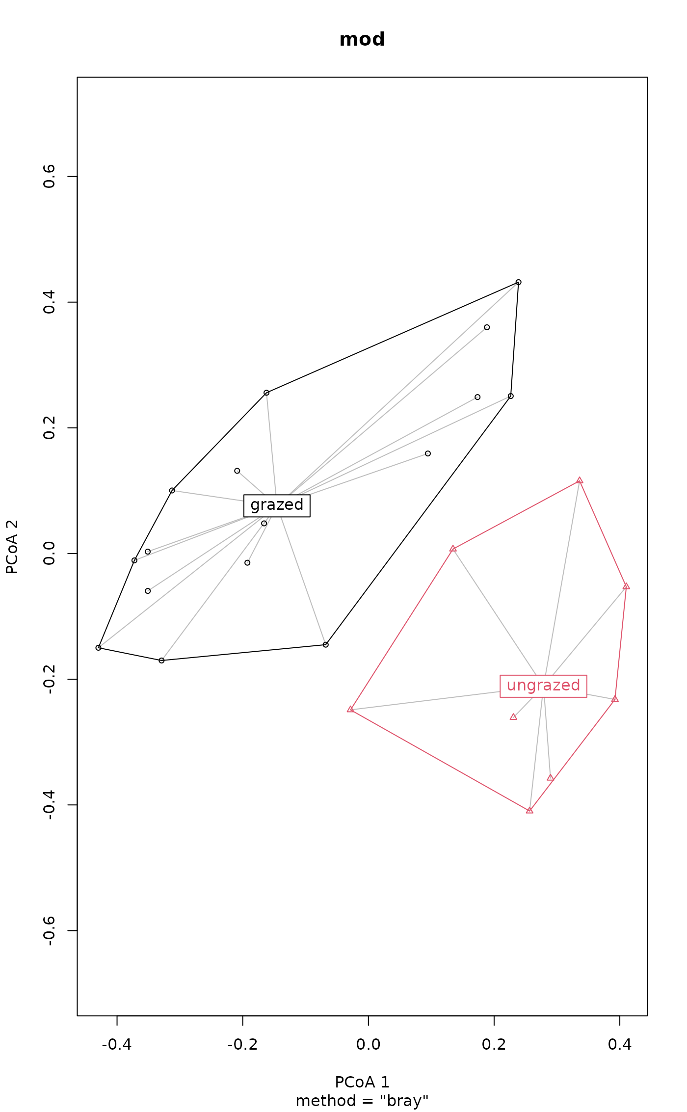
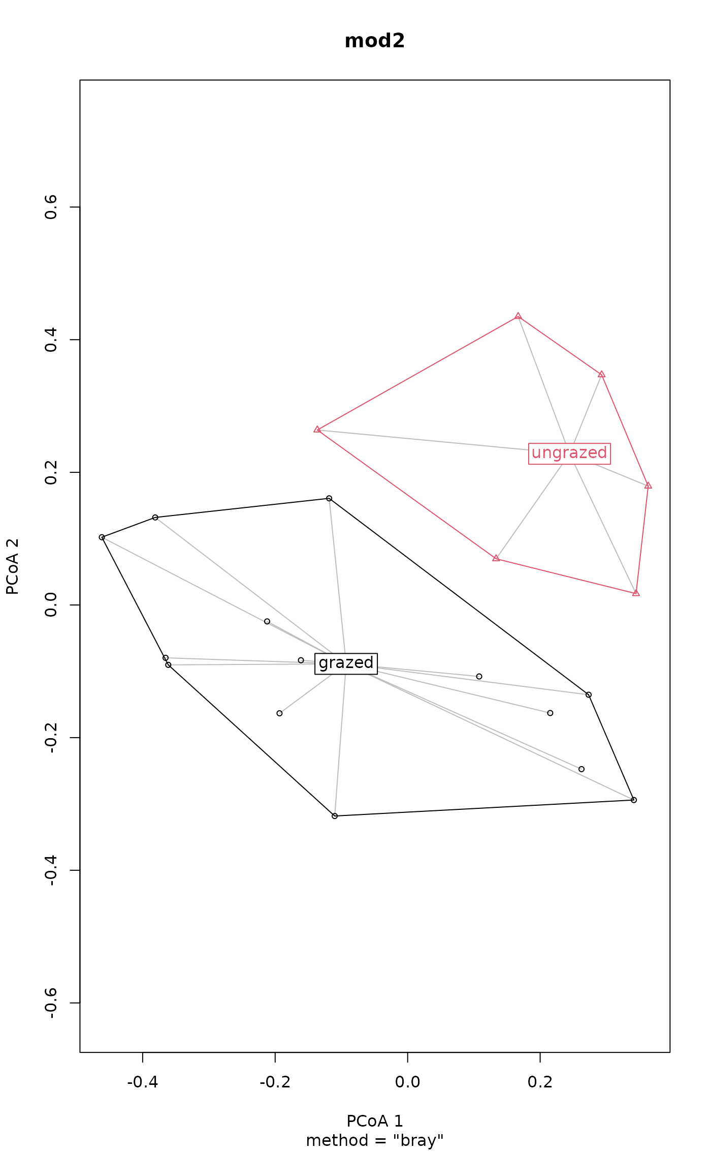
 ## Plot and show the groups and distances to centroids on the
## first two PCoA axes
plot(mod)
## Plot and show the groups and distances to centroids on the
## first two PCoA axes
plot(mod)
 betadistances(mod)
#> group nearest grazed ungrazed
#> 18 grazed grazed 0.3314940 0.4876932
#> 15 grazed grazed 0.2448593 0.6867177
#> 24 grazed grazed 0.4087618 0.7202852
#> 27 grazed grazed 0.4055027 0.6716925
#> 23 grazed grazed 0.2711717 0.5859224
#> 19 grazed grazed 0.3235683 0.4226658
#> 22 grazed grazed 0.3540192 0.7143106
#> 16 grazed grazed 0.3052699 0.6567417
#> 28 grazed grazed 0.5804799 0.8350802
#> 13 grazed grazed 0.4573620 0.5496107
#> 14 grazed grazed 0.4346688 0.7480122
#> 20 grazed grazed 0.2458315 0.5795502
#> 25 grazed grazed 0.3544958 0.7270236
#> 7 grazed grazed 0.5019108 0.6344208
#> 5 grazed grazed 0.6029360 0.7048208
#> 6 grazed grazed 0.4590746 0.5195341
#> 3 ungrazed ungrazed 0.5810524 0.2147308
#> 4 ungrazed ungrazed 0.5626172 0.4286653
#> 2 ungrazed ungrazed 0.6254225 0.1301314
#> 9 ungrazed ungrazed 0.6461171 0.2223194
#> 12 ungrazed ungrazed 0.5079965 0.0761938
#> 10 ungrazed ungrazed 0.6247805 0.1748861
#> 11 ungrazed ungrazed 0.3611882 0.3359708
#> 21 ungrazed grazed 0.5694430 0.5822677
## with data ellipses instead of hulls
plot(mod, ellipse = TRUE, hull = FALSE) # 1 sd data ellipse
betadistances(mod)
#> group nearest grazed ungrazed
#> 18 grazed grazed 0.3314940 0.4876932
#> 15 grazed grazed 0.2448593 0.6867177
#> 24 grazed grazed 0.4087618 0.7202852
#> 27 grazed grazed 0.4055027 0.6716925
#> 23 grazed grazed 0.2711717 0.5859224
#> 19 grazed grazed 0.3235683 0.4226658
#> 22 grazed grazed 0.3540192 0.7143106
#> 16 grazed grazed 0.3052699 0.6567417
#> 28 grazed grazed 0.5804799 0.8350802
#> 13 grazed grazed 0.4573620 0.5496107
#> 14 grazed grazed 0.4346688 0.7480122
#> 20 grazed grazed 0.2458315 0.5795502
#> 25 grazed grazed 0.3544958 0.7270236
#> 7 grazed grazed 0.5019108 0.6344208
#> 5 grazed grazed 0.6029360 0.7048208
#> 6 grazed grazed 0.4590746 0.5195341
#> 3 ungrazed ungrazed 0.5810524 0.2147308
#> 4 ungrazed ungrazed 0.5626172 0.4286653
#> 2 ungrazed ungrazed 0.6254225 0.1301314
#> 9 ungrazed ungrazed 0.6461171 0.2223194
#> 12 ungrazed ungrazed 0.5079965 0.0761938
#> 10 ungrazed ungrazed 0.6247805 0.1748861
#> 11 ungrazed ungrazed 0.3611882 0.3359708
#> 21 ungrazed grazed 0.5694430 0.5822677
## with data ellipses instead of hulls
plot(mod, ellipse = TRUE, hull = FALSE) # 1 sd data ellipse
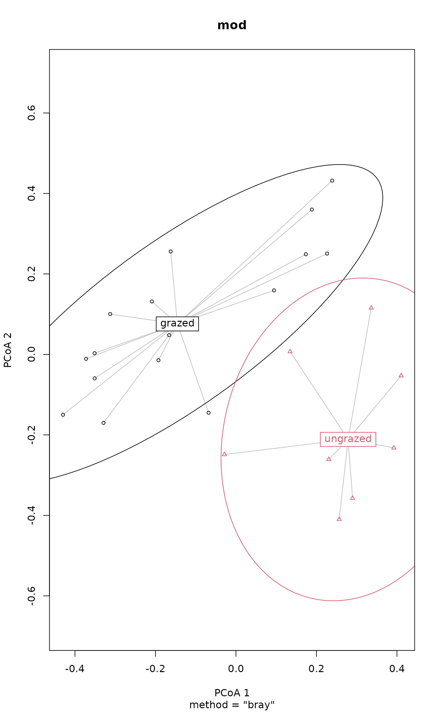
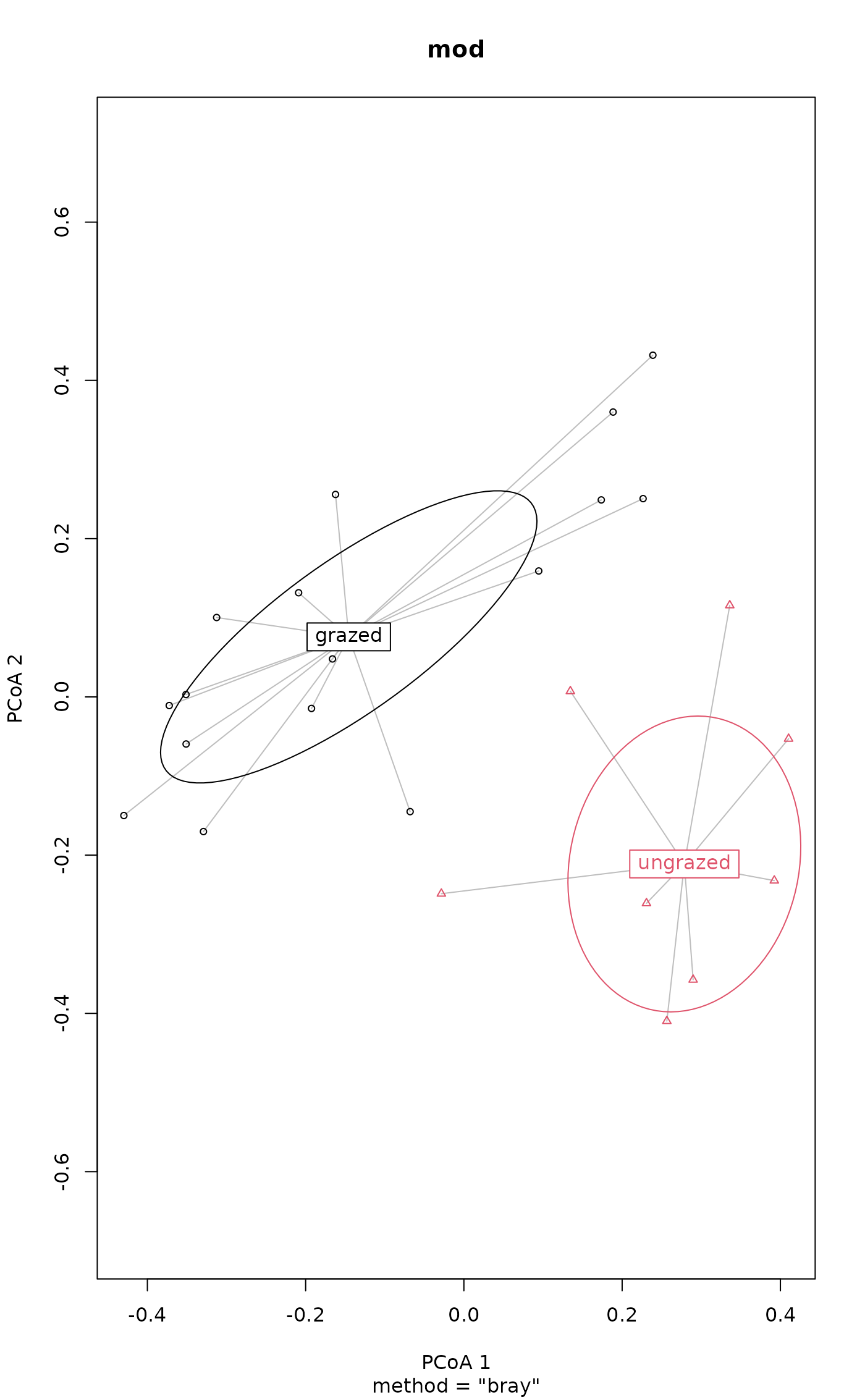 plot(mod, ellipse = TRUE, hull = FALSE, conf = 0.90) # 90% data ellipse
 # plot with manual colour specification
my_cols <- c("#1b9e77", "#7570b3")
plot(mod, col = my_cols, pch = c(16,17), cex = 1.1)
# plot with manual colour specification
my_cols <- c("#1b9e77", "#7570b3")
plot(mod, col = my_cols, pch = c(16,17), cex = 1.1)
 ## can also specify which axes to plot, ordering respected
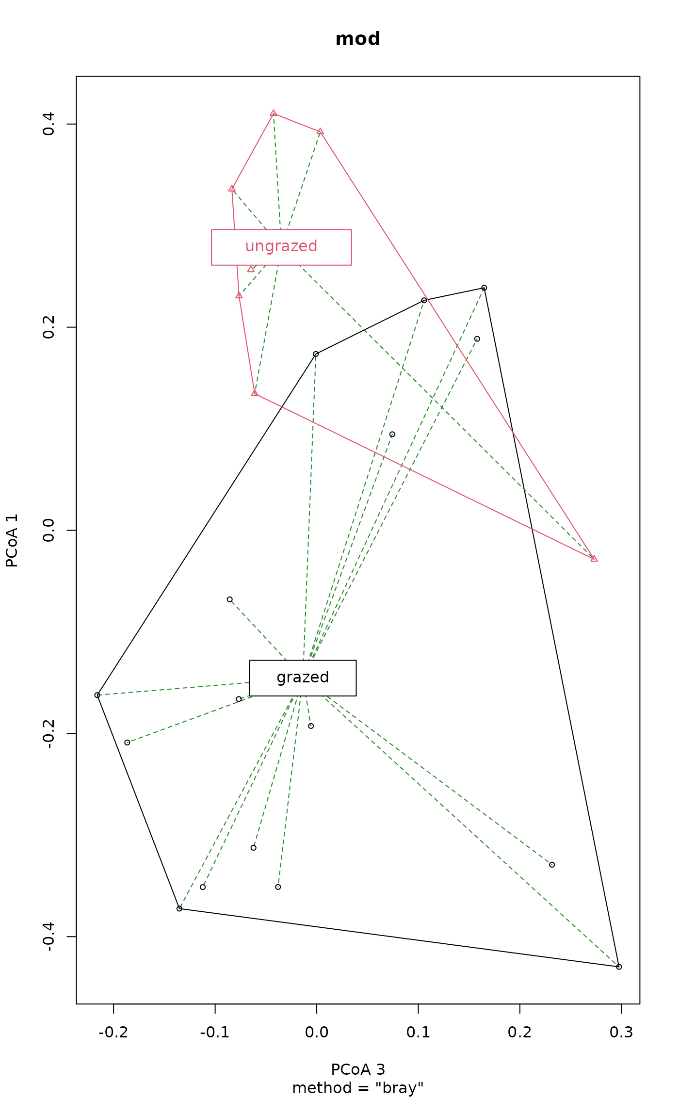
plot(mod, axes = c(3,1), seg.col = "forestgreen", seg.lty = "dashed")
## can also specify which axes to plot, ordering respected
plot(mod, axes = c(3,1), seg.col = "forestgreen", seg.lty = "dashed")
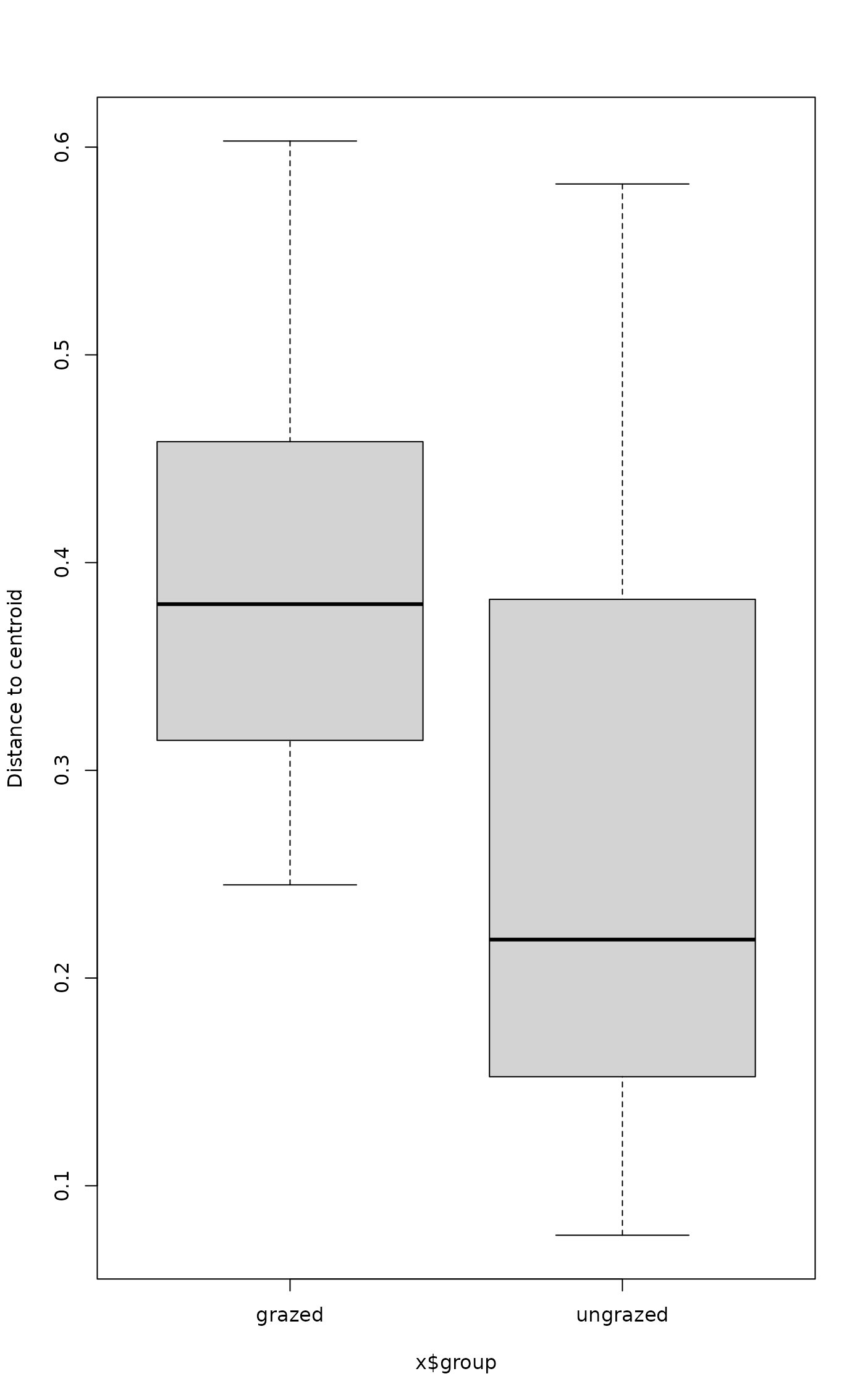
 ## Draw a boxplot of the distances to centroid for each group
boxplot(mod)
## Draw a boxplot of the distances to centroid for each group
boxplot(mod)
 ## `scores` and `eigenvals` also work
scrs <- scores(mod)
str(scrs)
#> List of 2
#> $ sites : num [1:24, 1:2] 0.0946 -0.3125 -0.3511 -0.3291 -0.1926 ...
#> ..- attr(*, "dimnames")=List of 2
#> .. ..$ : chr [1:24] "18" "15" "24" "27" ...
#> .. ..$ : chr [1:2] "PCoA1" "PCoA2"
#> $ centroids: num [1:2, 1:2] -0.1455 0.2786 0.0758 -0.2111
#> ..- attr(*, "dimnames")=List of 2
#> .. ..$ : chr [1:2] "grazed" "ungrazed"
#> .. ..$ : chr [1:2] "PCoA1" "PCoA2"
head(scores(mod, 1:4, display = "sites"))
#> PCoA1 PCoA2 PCoA3 PCoA4
#> 18 0.09459373 0.15914576 0.074400844 -0.202466025
#> 15 -0.31248809 0.10032751 -0.062243360 0.110844864
#> 24 -0.35106507 -0.05954096 -0.038079447 0.095060928
#> 27 -0.32914546 -0.17019348 0.231623720 0.019110623
#> 23 -0.19259443 -0.01459250 -0.005679372 -0.209718312
#> 19 -0.06794575 -0.14501690 -0.085645653 0.002431355
# group centroids/medians
scores(mod, 1:4, display = "centroids")
#> PCoA1 PCoA2 PCoA3 PCoA4
#> grazed -0.1455200 0.07584572 -0.01366220 -0.0178990
#> ungrazed 0.2786095 -0.21114993 -0.03475586 0.0220129
# eigenvalues from the underlying principal coordinates analysis
eigenvals(mod)
#> PCoA1 PCoA2 PCoA3 PCoA4 PCoA5 PCoA6 PCoA7
#> 1.7552165 1.1334455 0.4429018 0.3698054 0.2453532 0.1960921 0.1751131
#> PCoA8 PCoA9 PCoA10 PCoA11 PCoA12 PCoA13 PCoA14
#> 0.1284467 0.0971594 0.0759601 0.0637178 0.0583225 0.0394934 0.0172699
#> PCoA15 PCoA16 PCoA17 PCoA18 PCoA19 PCoA20 PCoA21
#> 0.0051011 -0.0004131 -0.0064654 -0.0133147 -0.0253944 -0.0375105 -0.0480069
#> PCoA22 PCoA23
#> -0.0537146 -0.0741390
## try out bias correction; compare with mod3
(mod3B <- betadisper(dis, groups, type = "median", bias.adjust=TRUE))
#>
#> Homogeneity of multivariate dispersions
#>
#> Call: betadisper(d = dis, group = groups, type = "median", bias.adjust
#> = TRUE)
#>
#> No. of Positive Eigenvalues: 15
#> No. of Negative Eigenvalues: 8
#>
#> Average distance to median:
#> grazed ungrazed
#> 0.4055 0.2893
#>
#> Eigenvalues for PCoA axes:
#> (Showing 8 of 23 eigenvalues)
#> PCoA1 PCoA2 PCoA3 PCoA4 PCoA5 PCoA6 PCoA7 PCoA8
#> 1.7552 1.1334 0.4429 0.3698 0.2454 0.1961 0.1751 0.1284
anova(mod3B)
#> Analysis of Variance Table
#>
#> Response: Distances
#> Df Sum Sq Mean Sq F value Pr(>F)
#> Groups 1 0.07193 0.071927 3.7826 0.06468 .
#> Residuals 22 0.41834 0.019015
#> ---
#> Signif. codes: 0 ‘***’ 0.001 ‘**’ 0.01 ‘*’ 0.05 ‘.’ 0.1 ‘ ’ 1
permutest(mod3B, permutations = 99)
#>
#> Permutation test for homogeneity of multivariate dispersions
#> Permutation: free
#> Number of permutations: 99
#>
#> Response: Distances
#> Df Sum Sq Mean Sq F N.Perm Pr(>F)
#> Groups 1 0.07193 0.071927 3.7826 99 0.05 *
#> Residuals 22 0.41834 0.019015
#> ---
#> Signif. codes: 0 ‘***’ 0.001 ‘**’ 0.01 ‘*’ 0.05 ‘.’ 0.1 ‘ ’ 1
## should always work for a single group
group <- factor(rep("grazed", NROW(varespec)))
(tmp <- betadisper(dis, group, type = "median"))
#>
#> Homogeneity of multivariate dispersions
#>
#> Call: betadisper(d = dis, group = group, type = "median")
#>
#> No. of Positive Eigenvalues: 15
#> No. of Negative Eigenvalues: 8
#>
#> Average distance to median:
#> grazed
#> 0.4255
#>
#> Eigenvalues for PCoA axes:
#> (Showing 8 of 23 eigenvalues)
#> PCoA1 PCoA2 PCoA3 PCoA4 PCoA5 PCoA6 PCoA7 PCoA8
#> 1.7552 1.1334 0.4429 0.3698 0.2454 0.1961 0.1751 0.1284
(tmp <- betadisper(dis, group, type = "centroid"))
#>
#> Homogeneity of multivariate dispersions
#>
#> Call: betadisper(d = dis, group = group, type = "centroid")
#>
#> No. of Positive Eigenvalues: 15
#> No. of Negative Eigenvalues: 8
#>
#> Average distance to centroid:
#> grazed
#> 0.4261
#>
#> Eigenvalues for PCoA axes:
#> (Showing 8 of 23 eigenvalues)
#> PCoA1 PCoA2 PCoA3 PCoA4 PCoA5 PCoA6 PCoA7 PCoA8
#> 1.7552 1.1334 0.4429 0.3698 0.2454 0.1961 0.1751 0.1284
## simulate missing values in 'd' and 'group'
## using spatial medians
groups[c(2,20)] <- NA
dis[c(2, 20)] <- NA
mod2 <- betadisper(dis, groups) ## messages
#> missing observations due to 'group' removed
#> missing observations due to 'd' removed
mod2
#>
#> Homogeneity of multivariate dispersions
#>
#> Call: betadisper(d = dis, group = groups)
#>
#> No. of Positive Eigenvalues: 14
#> No. of Negative Eigenvalues: 5
#>
#> Average distance to median:
#> grazed ungrazed
#> 0.3984 0.3008
#>
#> Eigenvalues for PCoA axes:
#> (Showing 8 of 19 eigenvalues)
#> PCoA1 PCoA2 PCoA3 PCoA4 PCoA5 PCoA6 PCoA7 PCoA8
#> 1.4755 0.8245 0.4218 0.3456 0.2159 0.1688 0.1150 0.1060
permutest(mod2, permutations = 99)
#>
#> Permutation test for homogeneity of multivariate dispersions
#> Permutation: free
#> Number of permutations: 99
#>
#> Response: Distances
#> Df Sum Sq Mean Sq F N.Perm Pr(>F)
#> Groups 1 0.039979 0.039979 2.4237 99 0.16
#> Residuals 18 0.296910 0.016495
anova(mod2)
#> Analysis of Variance Table
#>
#> Response: Distances
#> Df Sum Sq Mean Sq F value Pr(>F)
#> Groups 1 0.039979 0.039979 2.4237 0.1369
#> Residuals 18 0.296910 0.016495
plot(mod2)
## `scores` and `eigenvals` also work
scrs <- scores(mod)
str(scrs)
#> List of 2
#> $ sites : num [1:24, 1:2] 0.0946 -0.3125 -0.3511 -0.3291 -0.1926 ...
#> ..- attr(*, "dimnames")=List of 2
#> .. ..$ : chr [1:24] "18" "15" "24" "27" ...
#> .. ..$ : chr [1:2] "PCoA1" "PCoA2"
#> $ centroids: num [1:2, 1:2] -0.1455 0.2786 0.0758 -0.2111
#> ..- attr(*, "dimnames")=List of 2
#> .. ..$ : chr [1:2] "grazed" "ungrazed"
#> .. ..$ : chr [1:2] "PCoA1" "PCoA2"
head(scores(mod, 1:4, display = "sites"))
#> PCoA1 PCoA2 PCoA3 PCoA4
#> 18 0.09459373 0.15914576 0.074400844 -0.202466025
#> 15 -0.31248809 0.10032751 -0.062243360 0.110844864
#> 24 -0.35106507 -0.05954096 -0.038079447 0.095060928
#> 27 -0.32914546 -0.17019348 0.231623720 0.019110623
#> 23 -0.19259443 -0.01459250 -0.005679372 -0.209718312
#> 19 -0.06794575 -0.14501690 -0.085645653 0.002431355
# group centroids/medians
scores(mod, 1:4, display = "centroids")
#> PCoA1 PCoA2 PCoA3 PCoA4
#> grazed -0.1455200 0.07584572 -0.01366220 -0.0178990
#> ungrazed 0.2786095 -0.21114993 -0.03475586 0.0220129
# eigenvalues from the underlying principal coordinates analysis
eigenvals(mod)
#> PCoA1 PCoA2 PCoA3 PCoA4 PCoA5 PCoA6 PCoA7
#> 1.7552165 1.1334455 0.4429018 0.3698054 0.2453532 0.1960921 0.1751131
#> PCoA8 PCoA9 PCoA10 PCoA11 PCoA12 PCoA13 PCoA14
#> 0.1284467 0.0971594 0.0759601 0.0637178 0.0583225 0.0394934 0.0172699
#> PCoA15 PCoA16 PCoA17 PCoA18 PCoA19 PCoA20 PCoA21
#> 0.0051011 -0.0004131 -0.0064654 -0.0133147 -0.0253944 -0.0375105 -0.0480069
#> PCoA22 PCoA23
#> -0.0537146 -0.0741390
## try out bias correction; compare with mod3
(mod3B <- betadisper(dis, groups, type = "median", bias.adjust=TRUE))
#>
#> Homogeneity of multivariate dispersions
#>
#> Call: betadisper(d = dis, group = groups, type = "median", bias.adjust
#> = TRUE)
#>
#> No. of Positive Eigenvalues: 15
#> No. of Negative Eigenvalues: 8
#>
#> Average distance to median:
#> grazed ungrazed
#> 0.4055 0.2893
#>
#> Eigenvalues for PCoA axes:
#> (Showing 8 of 23 eigenvalues)
#> PCoA1 PCoA2 PCoA3 PCoA4 PCoA5 PCoA6 PCoA7 PCoA8
#> 1.7552 1.1334 0.4429 0.3698 0.2454 0.1961 0.1751 0.1284
anova(mod3B)
#> Analysis of Variance Table
#>
#> Response: Distances
#> Df Sum Sq Mean Sq F value Pr(>F)
#> Groups 1 0.07193 0.071927 3.7826 0.06468 .
#> Residuals 22 0.41834 0.019015
#> ---
#> Signif. codes: 0 ‘***’ 0.001 ‘**’ 0.01 ‘*’ 0.05 ‘.’ 0.1 ‘ ’ 1
permutest(mod3B, permutations = 99)
#>
#> Permutation test for homogeneity of multivariate dispersions
#> Permutation: free
#> Number of permutations: 99
#>
#> Response: Distances
#> Df Sum Sq Mean Sq F N.Perm Pr(>F)
#> Groups 1 0.07193 0.071927 3.7826 99 0.05 *
#> Residuals 22 0.41834 0.019015
#> ---
#> Signif. codes: 0 ‘***’ 0.001 ‘**’ 0.01 ‘*’ 0.05 ‘.’ 0.1 ‘ ’ 1
## should always work for a single group
group <- factor(rep("grazed", NROW(varespec)))
(tmp <- betadisper(dis, group, type = "median"))
#>
#> Homogeneity of multivariate dispersions
#>
#> Call: betadisper(d = dis, group = group, type = "median")
#>
#> No. of Positive Eigenvalues: 15
#> No. of Negative Eigenvalues: 8
#>
#> Average distance to median:
#> grazed
#> 0.4255
#>
#> Eigenvalues for PCoA axes:
#> (Showing 8 of 23 eigenvalues)
#> PCoA1 PCoA2 PCoA3 PCoA4 PCoA5 PCoA6 PCoA7 PCoA8
#> 1.7552 1.1334 0.4429 0.3698 0.2454 0.1961 0.1751 0.1284
(tmp <- betadisper(dis, group, type = "centroid"))
#>
#> Homogeneity of multivariate dispersions
#>
#> Call: betadisper(d = dis, group = group, type = "centroid")
#>
#> No. of Positive Eigenvalues: 15
#> No. of Negative Eigenvalues: 8
#>
#> Average distance to centroid:
#> grazed
#> 0.4261
#>
#> Eigenvalues for PCoA axes:
#> (Showing 8 of 23 eigenvalues)
#> PCoA1 PCoA2 PCoA3 PCoA4 PCoA5 PCoA6 PCoA7 PCoA8
#> 1.7552 1.1334 0.4429 0.3698 0.2454 0.1961 0.1751 0.1284
## simulate missing values in 'd' and 'group'
## using spatial medians
groups[c(2,20)] <- NA
dis[c(2, 20)] <- NA
mod2 <- betadisper(dis, groups) ## messages
#> missing observations due to 'group' removed
#> missing observations due to 'd' removed
mod2
#>
#> Homogeneity of multivariate dispersions
#>
#> Call: betadisper(d = dis, group = groups)
#>
#> No. of Positive Eigenvalues: 14
#> No. of Negative Eigenvalues: 5
#>
#> Average distance to median:
#> grazed ungrazed
#> 0.3984 0.3008
#>
#> Eigenvalues for PCoA axes:
#> (Showing 8 of 19 eigenvalues)
#> PCoA1 PCoA2 PCoA3 PCoA4 PCoA5 PCoA6 PCoA7 PCoA8
#> 1.4755 0.8245 0.4218 0.3456 0.2159 0.1688 0.1150 0.1060
permutest(mod2, permutations = 99)
#>
#> Permutation test for homogeneity of multivariate dispersions
#> Permutation: free
#> Number of permutations: 99
#>
#> Response: Distances
#> Df Sum Sq Mean Sq F N.Perm Pr(>F)
#> Groups 1 0.039979 0.039979 2.4237 99 0.16
#> Residuals 18 0.296910 0.016495
anova(mod2)
#> Analysis of Variance Table
#>
#> Response: Distances
#> Df Sum Sq Mean Sq F value Pr(>F)
#> Groups 1 0.039979 0.039979 2.4237 0.1369
#> Residuals 18 0.296910 0.016495
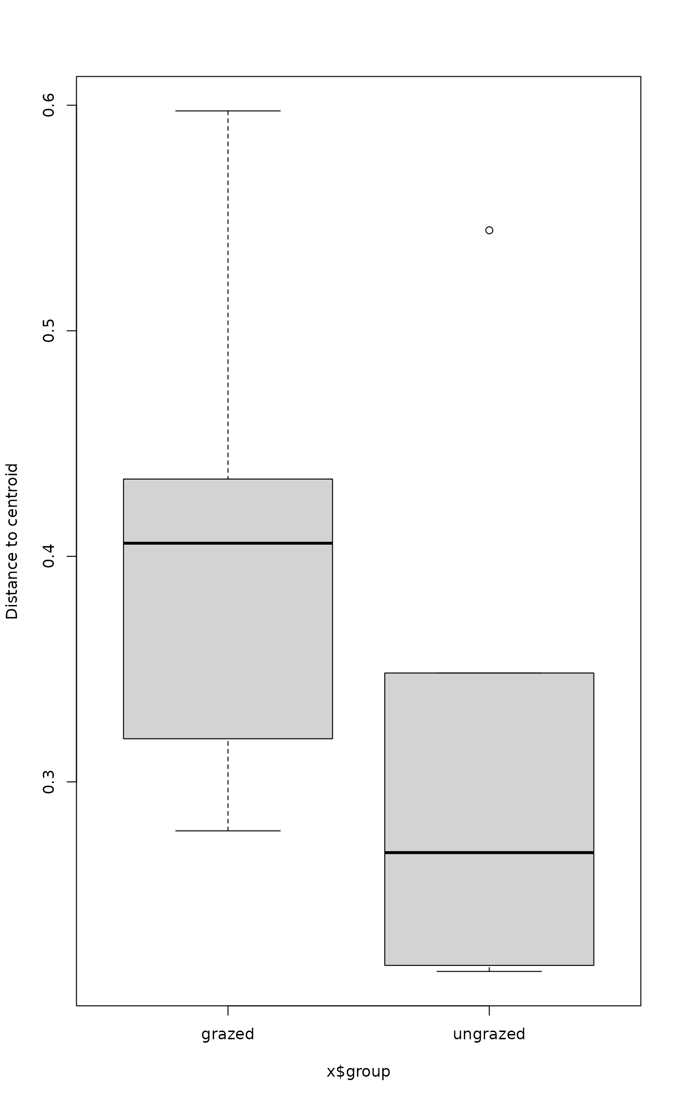
plot(mod2)
 boxplot(mod2)
 plot(TukeyHSD(mod2))
 ## Using group centroids
mod3 <- betadisper(dis, groups, type = "centroid")
#> missing observations due to 'group' removed
#> missing observations due to 'd' removed
mod3
#>
#> Homogeneity of multivariate dispersions
#>
#> Call: betadisper(d = dis, group = groups, type = "centroid")
#>
#> No. of Positive Eigenvalues: 14
#> No. of Negative Eigenvalues: 5
#>
#> Average distance to centroid:
#> grazed ungrazed
#> 0.4001 0.3108
#>
#> Eigenvalues for PCoA axes:
#> (Showing 8 of 19 eigenvalues)
#> PCoA1 PCoA2 PCoA3 PCoA4 PCoA5 PCoA6 PCoA7 PCoA8
#> 1.4755 0.8245 0.4218 0.3456 0.2159 0.1688 0.1150 0.1060
permutest(mod3, permutations = 99)
#>
#> Permutation test for homogeneity of multivariate dispersions
#> Permutation: free
#> Number of permutations: 99
#>
#> Response: Distances
#> Df Sum Sq Mean Sq F N.Perm Pr(>F)
#> Groups 1 0.033468 0.033468 3.1749 99 0.12
#> Residuals 18 0.189749 0.010542
anova(mod3)
#> Analysis of Variance Table
#>
#> Response: Distances
#> Df Sum Sq Mean Sq F value Pr(>F)
#> Groups 1 0.033468 0.033468 3.1749 0.09166 .
#> Residuals 18 0.189749 0.010542
#> ---
#> Signif. codes: 0 ‘***’ 0.001 ‘**’ 0.01 ‘*’ 0.05 ‘.’ 0.1 ‘ ’ 1
plot(mod3)
## Using group centroids
mod3 <- betadisper(dis, groups, type = "centroid")
#> missing observations due to 'group' removed
#> missing observations due to 'd' removed
mod3
#>
#> Homogeneity of multivariate dispersions
#>
#> Call: betadisper(d = dis, group = groups, type = "centroid")
#>
#> No. of Positive Eigenvalues: 14
#> No. of Negative Eigenvalues: 5
#>
#> Average distance to centroid:
#> grazed ungrazed
#> 0.4001 0.3108
#>
#> Eigenvalues for PCoA axes:
#> (Showing 8 of 19 eigenvalues)
#> PCoA1 PCoA2 PCoA3 PCoA4 PCoA5 PCoA6 PCoA7 PCoA8
#> 1.4755 0.8245 0.4218 0.3456 0.2159 0.1688 0.1150 0.1060
permutest(mod3, permutations = 99)
#>
#> Permutation test for homogeneity of multivariate dispersions
#> Permutation: free
#> Number of permutations: 99
#>
#> Response: Distances
#> Df Sum Sq Mean Sq F N.Perm Pr(>F)
#> Groups 1 0.033468 0.033468 3.1749 99 0.12
#> Residuals 18 0.189749 0.010542
anova(mod3)
#> Analysis of Variance Table
#>
#> Response: Distances
#> Df Sum Sq Mean Sq F value Pr(>F)
#> Groups 1 0.033468 0.033468 3.1749 0.09166 .
#> Residuals 18 0.189749 0.010542
#> ---
#> Signif. codes: 0 ‘***’ 0.001 ‘**’ 0.01 ‘*’ 0.05 ‘.’ 0.1 ‘ ’ 1
plot(mod3)
 boxplot(mod3)
 plot(TukeyHSD(mod3))
