Permutation Test for Constrained Correspondence Analysis, Redundancy Analysis and Constrained Analysis of Principal Coordinates

The function performs an ANOVA like permutation test for Constrained Correspondence Analysis (cca), Redundancy Analysis (rda) or distance-based Redundancy Analysis (dbRDA, dbrda) to assess the significance of constraints.

Usage

# S3 method for class 'cca'
anova(object, ..., permutations = how(nperm=999),
     by = NULL, model = c("reduced", "direct", "full"),
     parallel = getOption("mc.cores"), strata = NULL,
     cutoff = 1, scope = NULL, test = c("permutation", "F"))
# S3 method for class 'cca'
permutest(x, permutations = how(nperm = 99),
     model = c("reduced", "direct", "full"), by = NULL, first = FALSE,
     strata = NULL, parallel = getOption("mc.cores"), ...)

Arguments

object: One or several result objects from cca, rda, dbrda or capscale. For a single object, a test specified in by or an overall test is given. If there are several result objects, they should be nested, and they are compared against previous model in the order of nestedness.
x: A single ordination result object.
permutations: a list of control values for the permutations as returned by the function how, or the number of permutations required, or a permutation matrix where each row gives the permuted indices.
by: The default (NULL) performs overall test for the model. In permutest and anova you can set by = "term" for sequential test of terms (from first to last), and by = "onedf" for sequential test of one-degree-of-freedom contrasts of factor levels. In anova you can also set by = "margin" for marginal effecs of terms (each marginal term analysed in a model with all other variables), and by = "axis" for each constrained axis. Choices "terms" and "margin" can be used only with models fitted with formula. by cannot be used together with first = TRUE.
model: Permutation model: model="direct" permutes community data, model="reduced" permutes residuals of the community data after Conditions (partial model), model = "full" permutes residuals after Conditions and Constraints.
parallel: Use parallel processing with the given number of cores.
strata: An integer vector or factor specifying the strata for permutation. If supplied, observations are permuted only within the specified strata. It is an error to use this when permutations is a matrix, or a how defines blocks. This is a legacy argument: it is better to use permutations = how(..., blocks) instead.
cutoff: Only effective with by="axis" where stops permutations after an axis equals or exceeds the cutoff \(p\)-value.
scope: Only effective with by="margin" where it can be used to select the marginal terms for testing. The default is to test all marginal terms in drop.scope.
test: Test type, either permutation test or parametric \(F\)-test. Parametric test is only available for rda. It is similar as anova.mlm test = "Spherical" with Greenhouse-Geisser correction for asphericity.
first: Analyse only significance of the first axis.
...: Parameters passed to other functions. anova.cca passes all arguments to permutest.cca. In anova with by = "axis" you can use argument cutoff (defaults 1) which stops permutations after exceeding the given level.

Details

Functions anova.cca and permutest.cca implement ANOVA like permutation tests for the joint effect of constraints in cca, rda, dbrda or capscale. Function anova is intended as a more user-friendly alternative to permutest (that is the real workhorse).

Function anova can analyse a sequence of constrained ordination models. The analysis is based on the differences in residual deviance in permutations of nested models.

The default test is for the sum of all constrained eigenvalues. Setting first = TRUE will perform a test for the first constrained eigenvalue. Argument first can be set either in anova.cca or in permutest.cca. It is also possible to perform significance tests for each axis or for each term (constraining variable) using argument by in anova.cca. Setting by = "axis" will perform separate significance tests for each constrained axis (Legendre et al. 2011). You can stop permutation tests after exceeding a given significance level with argument cutoff to speed up calculations in large models. Setting by = "terms" will perform separate significance test for each term (constraining variable). The terms are assessed sequentially from first to last, and the order of the terms will influence their significances. Setting by = "onedf" will perform a similar sequential test for one-degree-of-freedom effects, where multi-level factors are split in their contrasts. Setting by = "margin" will perform separate significance test for each marginal term in a model with all other terms. The marginal test also accepts a scope argument for the drop.scope which can be a character vector of term labels that are analysed, or a fitted model of lower scope. The marginal effects are also known as “Type III” effects, but the current function only evaluates marginal terms. It will, for instance, ignore main effects that are included in interaction terms. In calculating pseudo-\(F\), all terms are compared to the same residual of the full model.

Community data are permuted with choice model="direct", and residuals after partial CCA/ RDA/ dbRDA with choice model="reduced" (default). If there is no partial CCA/ RDA/ dbRDA stage, model="reduced" simply permutes the data and is equivalent to model="direct". The test statistic is “pseudo-\(F\)”, which is the ratio of constrained and unconstrained total Inertia (Chi-squares, variances or something similar), each divided by their respective degrees of freedom. If there are no conditions (“partial” terms), the sum of all eigenvalues remains constant, so that pseudo-\(F\) and eigenvalues would give equal results. In partial CCA/ RDA/ dbRDA, the effect of conditioning variables (“covariables”) is removed before permutation, and the total Chi-square is not fixed, and test based on pseudo-\(F\) would differ from the test based on plain eigenvalues.

Function can also perform parametric \(F\)-test on rda models. This test is similar to test = "Spherical" in anova.mlm. The test uses the tabulated \(F\)-values but multiplies the degrees of freedom with number of variables (species, columns) times correction factor epsilon, using Greenhouse-Geisser correction for asphericity. Preliminary tests indicate that this test is often consistent with permutation tests in rda (but not in cca and cannot be used with distance-based methods). However, if you use this test, it is best to check that it gives consistent results with permutation tests (see Examples).

Value

The function anova.cca calls permutest.cca and fills an anova table. Additional attributes are Random.seed (the random seeds used), control (the permutation design, see how) and F.perm (the permuted test statistics).

References

Legendre, P. and Legendre, L. (2012). Numerical Ecology. 3rd English ed. Elsevier.

Legendre, P., Oksanen, J. and ter Braak, C.J.F. (2011). Testing the significance of canonical axes in redundancy analysis. Methods in Ecology and Evolution 2, 269–277.

Author

Jari Oksanen

Examples

data(dune, dune.env)
mod <- cca(dune ~ Moisture + Management, dune.env)

## overall test
anova(mod)
#> Permutation test for cca under reduced model
#> Permutation: free
#> Number of permutations: 999
#> 
#> Model: cca(formula = dune ~ Moisture + Management, data = dune.env)
#>          Df ChiSquare      F Pr(>F)   
#> Model     6    1.0024 1.9515  0.003 **
#> Residual 13    1.1129                 
#> ---
#> Signif. codes:  0 ‘***’ 0.001 ‘**’ 0.01 ‘*’ 0.05 ‘.’ 0.1 ‘ ’ 1

## tests for individual terms and contrasts
anova(mod, by = "term")
#> Permutation test for cca under reduced model
#> Terms added sequentially (first to last)
#> Permutation: free
#> Number of permutations: 999
#> 
#> Model: cca(formula = dune ~ Moisture + Management, data = dune.env)
#>            Df ChiSquare      F Pr(>F)    
#> Moisture    3   0.62831 2.4465  0.001 ***
#> Management  3   0.37407 1.4565  0.049 *  
#> Residual   13   1.11289                  
#> ---
#> Signif. codes:  0 ‘***’ 0.001 ‘**’ 0.01 ‘*’ 0.05 ‘.’ 0.1 ‘ ’ 1
anova(mod, by = "margin")
#> Permutation test for cca under reduced model
#> Marginal effects of terms
#> Permutation: free
#> Number of permutations: 999
#> 
#> Model: cca(formula = dune ~ Moisture + Management, data = dune.env)
#>            Df ChiSquare      F Pr(>F)  
#> Moisture    3   0.39854 1.5518  0.036 *
#> Management  3   0.37407 1.4565  0.053 .
#> Residual   13   1.11289                
#> ---
#> Signif. codes:  0 ‘***’ 0.001 ‘**’ 0.01 ‘*’ 0.05 ‘.’ 0.1 ‘ ’ 1
anova(mod, by = "onedf")
#> Permutation test for cca under reduced model
#> Sequential test for contrasts
#> Permutation: free
#> Number of permutations: 999
#> 
#> Model: cca(formula = dune ~ Moisture + Management, data = dune.env)
#>              Df ChiSquare      F Pr(>F)    
#> Moisture.L    1   0.41081 4.7988  0.001 ***
#> Moisture.Q    1   0.11261 1.3154  0.167    
#> Moisture.C    1   0.10489 1.2253  0.226    
#> ManagementHF  1   0.08849 1.0337  0.359    
#> ManagementNM  1   0.20326 2.3744  0.011 *  
#> ManagementSF  1   0.08231 0.9615  0.455    
#> Residual     13   1.11289                  
#> ---
#> Signif. codes:  0 ‘***’ 0.001 ‘**’ 0.01 ‘*’ 0.05 ‘.’ 0.1 ‘ ’ 1

## compare several models in succession
mod0 <- cca(dune ~ 1, dune.env)
mod1 <- cca(dune ~ Moisture + A1, dune.env)
mod2 <- update(mod1, . ~ . + Management + Manure, dune.env)
#> 
#> Some constraints or conditions were aliased because they were redundant. This
#> can happen if terms are constant or linearly dependent (collinear): ‘Manure^4’
anova(mod0, mod1, mod2)
#> Permutation tests for cca under reduced model
#> Permutation: free
#> Number of permutations: 999
#> 
#> Model 1: dune ~ 1
#> Model 2: dune ~ Moisture + A1
#> Model 3: dune ~ Moisture + A1 + Management + Manure
#>   ResDf ResChiSquare Df ChiSquare      F Pr(>F)   
#> 1    19       2.1153                              
#> 2    15       1.3715  4   0.74374 2.2546  0.003 **
#> 3     9       0.7422  6   0.62933 1.2719  0.105   
#> ---
#> Signif. codes:  0 ‘***’ 0.001 ‘**’ 0.01 ‘*’ 0.05 ‘.’ 0.1 ‘ ’ 1

## See that permutation and F-distribution are consistent
mod <- rda(dune ~ Moisture + Management, dune.env)
(ano <- anova(mod))
#> Permutation test for rda under reduced model
#> Permutation: free
#> Number of permutations: 999
#> 
#> Model: rda(formula = dune ~ Moisture + Management, data = dune.env)
#>          Df Variance      F Pr(>F)    
#> Model     6   46.425 2.6682  0.001 ***
#> Residual 13   37.699                  
#> ---
#> Signif. codes:  0 ‘***’ 0.001 ‘**’ 0.01 ‘*’ 0.05 ‘.’ 0.1 ‘ ’ 1
anova(mod, test = "F")
#> Parametric F-test for rda  
#> Greenhouse-Geisser epsilon: 0.245 
#> 
#> Model: rda(formula = dune ~ Moisture + Management, data = dune.env)
#>          Df Variance      F    Pr(>F)    
#> Model     6   46.425 2.6682 3.256e-05 ***
#> Residual 13   37.699                     
#> ---
#> Signif. codes:  0 ‘***’ 0.001 ‘**’ 0.01 ‘*’ 0.05 ‘.’ 0.1 ‘ ’ 1
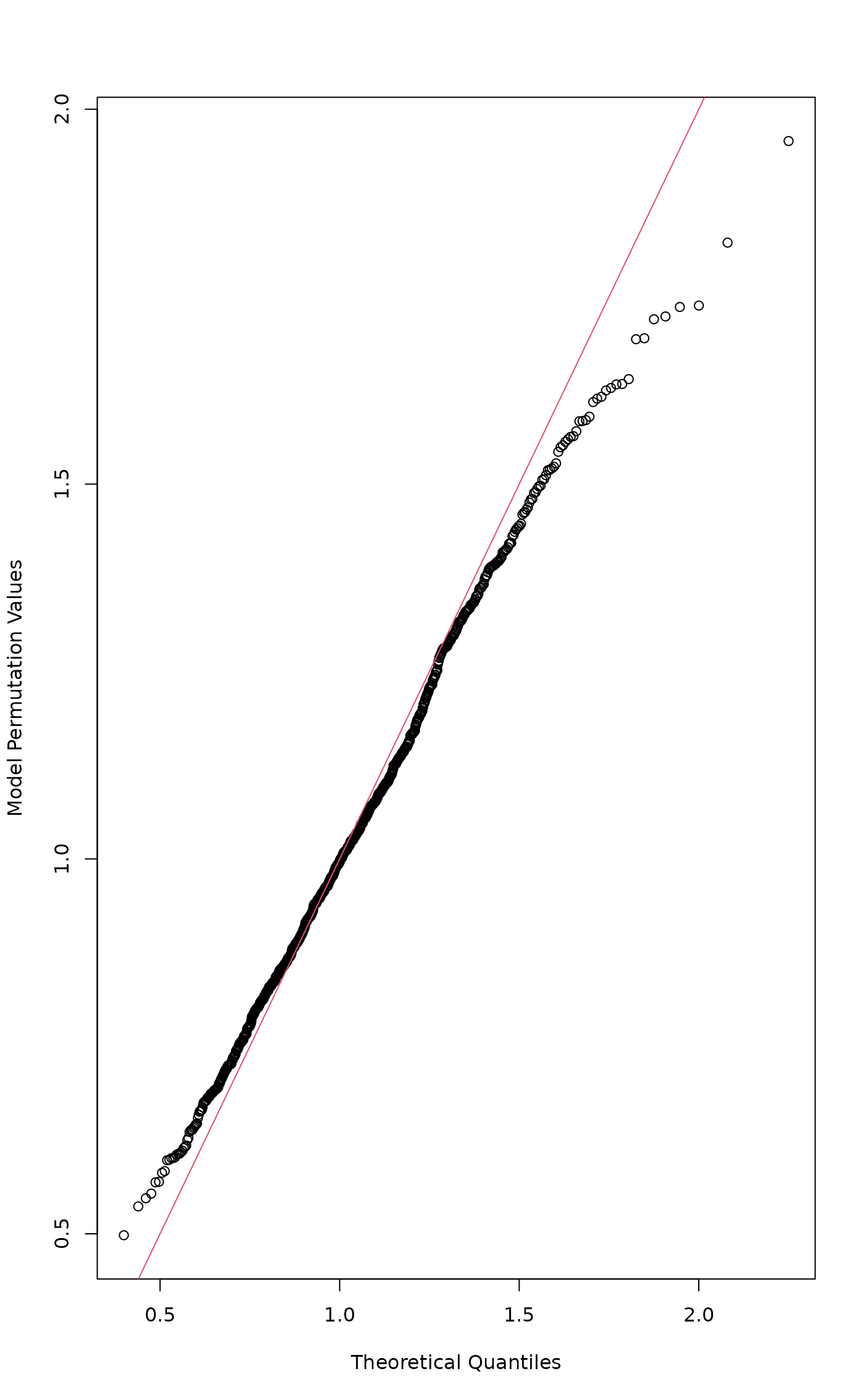
## adjustment for degrees of freedom in F distribution
adj <- ncol(dune) * 0.245 # Greenhouse-Geisser epsilon
qqnorm(permustats(ano), x = qf(ppoints(999), 6*adj, 13*adj, lower.tail=FALSE),
  observed = FALSE)
abline(0, 1, col = 2) # line of equality