Display Compact Ordered Community Tables

Functions vegemite and tabasco display compact community tables. Function vegemite prints text tables where species are rows, and each site takes only one column without spaces. Function tabasco provides interface for heatmap for a colour image of the data. The community table can be ordered by explicit indexing, by environmental variables or results from an ordination or cluster analysis.

Usage

vegemite(x, use, scale, sp.ind, site.ind, zero=".", select,
    diagonalize = FALSE, ...)
tabasco(x, use, sp.ind = NULL, site.ind = NULL, select,
    Rowv = TRUE, Colv = TRUE, labRow = NULL, labCol = NULL,
    scale, col = heat.colors(12), ...)
coverscale(x, scale=c("Braun.Blanquet", "Domin", "Hult", "Hill", "fix","log"),
           maxabund, character = TRUE)

Arguments

x: Community data.
use: Either a numeric vector or a classification factor, or an object from cca, decorana etc. or hclust or a dendrogram for ordering sites and species.
sp.ind, site.ind: Species and site indices. In tabasco, these can also be hclust tree, agnes clusterings or dendrograms.
zero: Character used for zeros.
select: Select a subset of sites. This can be a logical vector (TRUE for selected sites), or a vector of indices of selected sites. The order of indices does not influence results, but you must specify use or site.ind to reorder sites.
diagonalize: Try to re-order vegemite table to a diagonal pattern when using classification factor or a dendrogram. Dendrograms are re-orded by the first axis of correspondence analysis. Factor levels and sites within factor levels are re-ordered by the first axis of (constrained) correspondence analysis.
Rowv, Colv: Re-order factors or dendrograms for the rows (sites) or columns (species) of x. If Rowv = TRUE, factor levels and sites within factors are re-ordered to show diagonal pattern using CCA. If Rowv = TRUE, row dendrograms are ordered by the first axis of correspondence analysis, and when Colv = TRUE column dendrograms by the weighted average (wascores) of the row order. Alternatively, the arguments can be vectors that are used to reorder the dendrogram.
labRow, labCol: character vectors with row and column labels used in the heatmap instead of the default. NB., the input matrix is transposed so that row labels will be used for data columns.
scale: In vegemite and coverscale: cover scale used (can be abbreviated). In tabasco: scaling of colours in heatmap. The alternatives of coverscale can be used in tabasco, and in addition "column" or "row" scale columns or rows to equal maxima (NB., these refer to the transposed data of the heatmap), while "none" uses original values.
col: A vector of colours used for above-zero abundance values.
maxabund: Maximum abundance used with scale = "log". Data maximum in the selected subset will be used if this is missing.
character: Return character codes suitable for tabulation in vegemite. If FALSE, returns corresponding integers suitable for numerical analysis.
...: Arguments passed to coverscale (i.e., maxabund) in vegemite and to heatmap in tabasco.

Details

The function vegemite prints a traditional community table. The display is transposed, so that species are in rows and sites in columns. The table is printed in compact form: only one character can be used for abundance, and there are no spaces between columns. Species with no occurrences are dropped from the table.

Function tabasco produces a similar table as vegemite using heatmap, where abundances are coded by colours. The function scales the abundances to equal intervals for colour palette, but either rows or columns can be scaled to equal maxima, or the coverscale class systems can be used. The function can also display dendrograms for sites (columns) or species if these are given as an argument (use for sites, sp.ind for species).

The parameter use will be used to re-order output. The use can be a vector or an object from hclust or agnes, a dendrogram or any ordination result recognized by scores (all ordination methods in vegan and some of those not in vegan). The hclust, agnes and dendrogram must be for sites. The dendrogram is displayed above the sites in tabasco, but is not shown in vegemite. In tabasco the species dendrogram can be given in sp.ind.

If use is a numeric vector, it is used for ordering sites, and if it is a factor, it is used to order sites by classes. If use is an object from ordination, both sites and species are arranged by the first axis (provided that results are available also for species). When use is an object from hclust, agnes or a dendrogram, the sites are ordered similarly as in the cluster dendrogram. Function tabasco re-orders the dendrogram to give a diagonal pattern if Rowv = TRUE. Alternatively, if Rowv is a vector its values are used to re-order dendrogram. With diagonalize = TRUE the dendrogram will be re-ordered in vegemite to give a diagonal pattern. If use is a factor, its levels and sites within levels will be reordered to give a diagonal pattern if diagonalize = TRUE in vegemite or Rowv = TRUE in tabasco. In all cases where species scores are missing, species are ordered by their weighted averages (wascores) on site order or site value.

Species and sites can be ordered explicitly giving their indices or names in parameters sp.ind and site.ind. If these are given, they take precedence over use. A subset of sites can be displayed using argument select, but this cannot be used to order sites, but you still must give use or site.ind. However, tabasco makes two exceptions: site.ind and select cannot be used when use is a dendrogram (clustering result). In addition, the sp.ind can be an hclust tree, agnes clustering or a dendrogram, and in that case the dendrogram is plotted on the left side of the heatmap. Phylogenetic trees cannot be directly used, but package ape has tools to transform these to hclust trees.

If scale is given, vegemite calls coverscale to transform percent cover scale or some other scales into traditional class scales used in vegetation science (coverscale can be called directly, too). Function tabasco can also use these traditional class scales, but it treats the transformed values as corresponding integers. Braun-Blanquet and Domin scales are actually not strict cover scales, and the limits used for codes r and + are arbitrary. Scale Hill may be inappropriately named, since Mark O. Hill probably never intended this as a cover scale. However, it is used as default “cut levels” in his TWINSPAN, and surprisingly many users stick to this default, and this is a de facto standard in publications. All traditional scales assume that values are cover percentages with maximum 100. However, non-traditional alternative log can be used with any scale range. Its class limits are integer powers of 1/2 of the maximum (argument maxabund), with + used for non-zero entries less than 1/512 of the maximum (log stands alternatively for logarithmic or logical). Scale fix is intended for “fixing” 10-point scales: it truncates scale values to integers, and replaces 10 with X and positive values below 1 with +.

Value

The functions are used mainly to display a table, but they return (invisibly) a list with items species for ordered species index, sites for ordered site index, and table for the final ordered community table.

These items can be used as arguments sp.ind and site.ind to reproduce the table, or the table can be further edited. In addition to the table, vegemite prints the numbers of species and sites and the name of the used cover scale.

References

The cover scales are presented in many textbooks of vegetation science; I used:

Shimwell, D.W. (1971) The Description and Classification of Vegetation. Sidgwick & Jackson.

Author

Jari Oksanen

Note

The name vegemite was chosen because the output is so compact, and the tabasco because it is just as compact, but uses heat colours.

Examples

data(varespec)
## Print only more common species
freq <- apply(varespec > 0, 2, sum)
vegemite(varespec, scale="Hult", sp.ind = freq > 10)
#>                                   
#>           1122212121122       1112
#>           854739268340575634292011
#>  Callvulg 111...11.311...1111.111.
#>  Empenigr 211332121112211111212213
#>  Vaccviti 323332212113221211233234
#>  Pinusylv 111.111111111.11.1111111
#>  Dicrfusc 12.111441121211111111111
#>  Dicrpoly .11.11.11..1.11....1.111
#>  Pleuschr 144533435123411111111131
#>  Polyjuni 111.11.111112111.111.111
#>  Pohlnuta 111111111111.1..11.11111
#>  Ptilcili 1111111111..1..11.11..12
#>  Cladarbu 321122121332143423111121
#>  Cladrang 321221131312145443313241
#>  Cladstel 11111311.211.11254555542
#>  Cladunci 112111111131111111111111
#>  Cladcocc 11..11111111111111.1.11.
#>  Cladcorn 111111111111111111111111
#>  Cladgrac 111111111111111111111.11
#>  Cladfimb 11.1111111111111111111.1
#>  Cladcris 111111111111111111111111
#>  Cladchlo ..1.111..1...1.11.11.1.1
#>  Cetreric 111...11.111111111.1.1..
#>  Cetrisla .11....1111.1....1.11111
#>  Stersp   111.11.1111.112111...11.
#>  Claddefo 1111111111111111111111.1
#> 24 sites, 24 species
#> scale:  Hult 
## Order by correspondence analysis, use Hill scaling and layout:
dca <- decorana(varespec)
vegemite(varespec, dca, "Hill", zero="-")
#>                                   
#>            1   1  1 11122211122222
#>           203942561738913046572458
#>  Flavniva -1114-11-1-11-1---------
#>  Cladstel 5555551451425411111211--
#>  Cladphyl -1-1----1-------1-------
#>  Cladcerv 1---1-----------------1-
#>  Cladsp   ---11--1--11---1-1-11-1-
#>  Cladamau --1---1----1------------
#>  Cladchlo 1111---1-11-111-----11--
#>  Cladrang 535254555555223414332321
#>  Diphcomp --11-----112----------1-
#>  Stersp   -11-1-4111111-1-111--111
#>  Pinusylv 11-111111-111111111-1111
#>  Polypili ------111--11-11--1-----
#>  Cetrisla -1-111--1-1--1--111--111
#>  Cladcocc -1111-1111111-11111-1-11
#>  Cladarbu 113142453555313343413231
#>  Vacculig --1-1----3-1---1---12-11
#>  Pohlnuta -11111--11111111111111-1
#>  Cladfimb 11111111-111111111111-11
#>  Callvulg 111-21-12-51---1221-21--
#>  Icmaeric ------1--1------11------
#>  Empenigr 342214131314344333143131
#>  Vaccviti 342514244334455432444443
#>  Cladgrac 1-1111111111111111111111
#>  Cetreric -1111-11-111---1111-111-
#>  Cladcorn 111111111111111111111111
#>  Cladcris 111111111111111111111111
#>  Peltapht --------1-11--1----1--1-
#>  Ptilcili 1-11---11-11141--1111111
#>  Barbhatc ----------1-121----1----
#>  Claddefo 11111111-111111111111111
#>  Cladbotr ----------1-1111---1-1-1
#>  Betupube -------------1------1-1-
#>  Dicrpoly -1-1--1-11--1211-11--1-1
#>  Cladunci 111111122111111251212311
#>  Polycomm ------------11--1--1--1-
#>  Polyjuni 11-11-1111111121111--131
#>  Rhodtome ----------1--2-----21--1
#>  Dicrfusc 111111111121112145425-41
#>  Pleuschr 111213114132524434555555
#>  Vaccmyrt ---1------1-24--12133--4
#>  Descflex ----1----1--11-----21-11
#>  Nepharct --1------1-1---1------2-
#>  Dicrsp   -----1----1--1-1-11-1541
#>  Hylosple ---------------1---3--13
#> 24 sites, 44 species
#> scale:  Hill 
## Show one class from cluster analysis, but retain the ordering above
clus <- hclust(vegdist(varespec))
cl <- cutree(clus, 3)
sel <- vegemite(varespec, use=dca, select = cl == 3, scale="Br")
#>                
#>            1 12
#>           20921
#>  Flavniva .++..
#>  Cladstel 55542
#>  Cladphyl .++..
#>  Cladcerv r....
#>  Cladsp   ..+..
#>  Cladchlo r++.+
#>  Cladrang 22121
#>  Diphcomp ..+..
#>  Stersp   .+...
#>  Pinusylv r++1+
#>  Cetrisla .++++
#>  Cladcocc .++..
#>  Cladarbu +1+1+
#>  Pohlnuta .++++
#>  Cladfimb r++++
#>  Callvulg r+.+.
#>  Empenigr 22122
#>  Vaccviti 22223
#>  Cladgrac r.+++
#>  Cetreric .++..
#>  Cladcorn r+++r
#>  Cladcris r++++
#>  Ptilcili r.+.2
#>  Barbhatc ....1
#>  Claddefo r++++
#>  Cladbotr ....+
#>  Betupube ....+
#>  Dicrpoly .++.1
#>  Cladunci +++1+
#>  Polycomm ....+
#>  Polyjuni r++.+
#>  Rhodtome ....1
#>  Dicrfusc r++++
#>  Pleuschr ++121
#>  Vaccmyrt ..+.2
#>  Descflex ....+
#>  Dicrsp   ...++
#> 5 sites, 37 species
#> scale:  Braun.Blanquet 
## Re-create previous
vegemite(varespec, sp=sel$sp, site=sel$site, scale="Hult")
#>                
#>            1 12
#>           20921
#>  Flavniva .11..
#>  Cladstel 55552
#>  Cladphyl .11..
#>  Cladcerv 1....
#>  Cladsp   ..1..
#>  Cladchlo 111.1
#>  Cladrang 32131
#>  Diphcomp ..1..
#>  Stersp   .1...
#>  Pinusylv 11111
#>  Cetrisla .1111
#>  Cladcocc .11..
#>  Cladarbu 11111
#>  Pohlnuta .1111
#>  Cladfimb 11111
#>  Callvulg 11.1.
#>  Empenigr 22123
#>  Vaccviti 22334
#>  Cladgrac 1.111
#>  Cetreric .11..
#>  Cladcorn 11111
#>  Cladcris 11111
#>  Ptilcili 1.1.2
#>  Barbhatc ....1
#>  Claddefo 11111
#>  Cladbotr ....1
#>  Betupube ....1
#>  Dicrpoly .11.1
#>  Cladunci 11111
#>  Polycomm ....1
#>  Polyjuni 111.1
#>  Rhodtome ....1
#>  Dicrfusc 11111
#>  Pleuschr 11111
#>  Vaccmyrt ..1.3
#>  Descflex ....1
#>  Dicrsp   ...11
#> 5 sites, 37 species
#> scale:  Hult 
## Re-order clusters by ordination
clus <- as.dendrogram(clus)
clus <- reorder(clus, scores(dca, choices=1, display="sites"), agglo.FUN = mean)
vegemite(varespec, clus, scale = "Hult")
#>                                   
#>             1   111  1211221212222
#>           431567380922149306254578
#>  Cladamau .1.1...1................
#>  Flavniva 21.111.111....11........
#>  Cladphyl ..1.....11...1..........
#>  Diphcomp .1...111.1...........1..
#>  Cladstel 454121215555213111111.1.
#>  Cladrang 344544332133111223121121
#>  Cladarbu 322344331111132222121111
#>  Icmaeric ...1.1.......1...1......
#>  Callvulg 111.1.311.11.1..11111...
#>  Polypili ..111..1......111..1....
#>  Nepharct .1...1.1........1....1..
#>  Stersp   111211111....111.1.111.1
#>  Cladchlo .1..111.111.1.11..1.1...
#>  Cladcerv 1.........1..........1..
#>  Cetreric 11.1111111...1..111111..
#>  Cladcocc 1111111111...1111111.1.1
#>  Cladcorn 111111111111111111111111
#>  Cladcris 111111111111111111111111
#>  Cladfimb 11.11111111111111111.111
#>  Cladgrac 11111111.111111111111111
#>  Polyjuni 1.111111111.111111.112.1
#>  Vacculig 11...2.1........1.1..111
#>  Pinusylv 1.111.1111111111111111.1
#>  Pohlnuta 111..11111.1111111111.11
#>  Claddefo 11.111111111111111111111
#>  Cladunci 111111111111131111112111
#>  Cladsp   1...1.11.1......111..11.
#>  Peltapht ..1...11.......1.....11.
#>  Vaccviti 113122132323412331223232
#>  Cetrisla 1.1...1.11.111...1.111.1
#>  Dicrpoly ..11.1..11..1.1111.11..1
#>  Empenigr 111111122122312322111231
#>  Ptilcili .11.1.11.11.2.11.1111111
#>  Dicrfusc 11111111111112111442.211
#>  Barbhatc ......1.....1.11......1.
#>  Descflex 1....1......1.1...1..111
#>  Pleuschr 113111111111123333444455
#>  Vaccmyrt ......1..1..311..111..13
#>  Cladbotr ......1.....1.111...1.11
#>  Rhodtome ......1.....1.....1...11
#>  Polycomm ............111......11.
#>  Betupube ............1.....1..1..
#>  Dicrsp   ......1....11...111133.1
#>  Hylosple ................1....122
#> 24 sites, 44 species
#> scale:  Hult 

## Abundance values have such a wide range that they must be rescaled
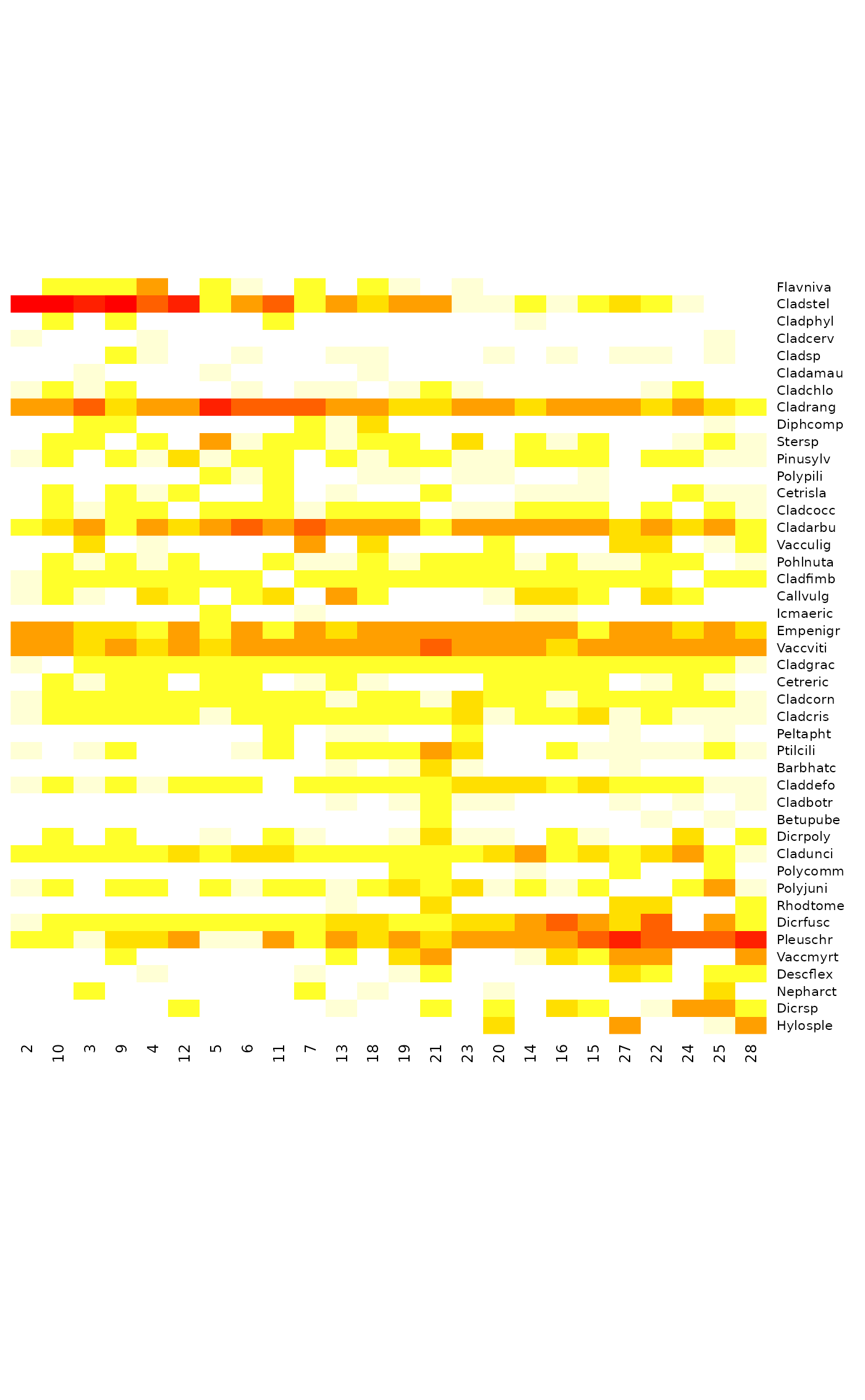
tabasco(varespec, dca, scale="Braun")


## Classification trees for species
data(dune, dune.taxon)
taxontree <- hclust(taxa2dist(dune.taxon))
plotree <- hclust(vegdist(dune), "average")
## Automatic reordering of clusters
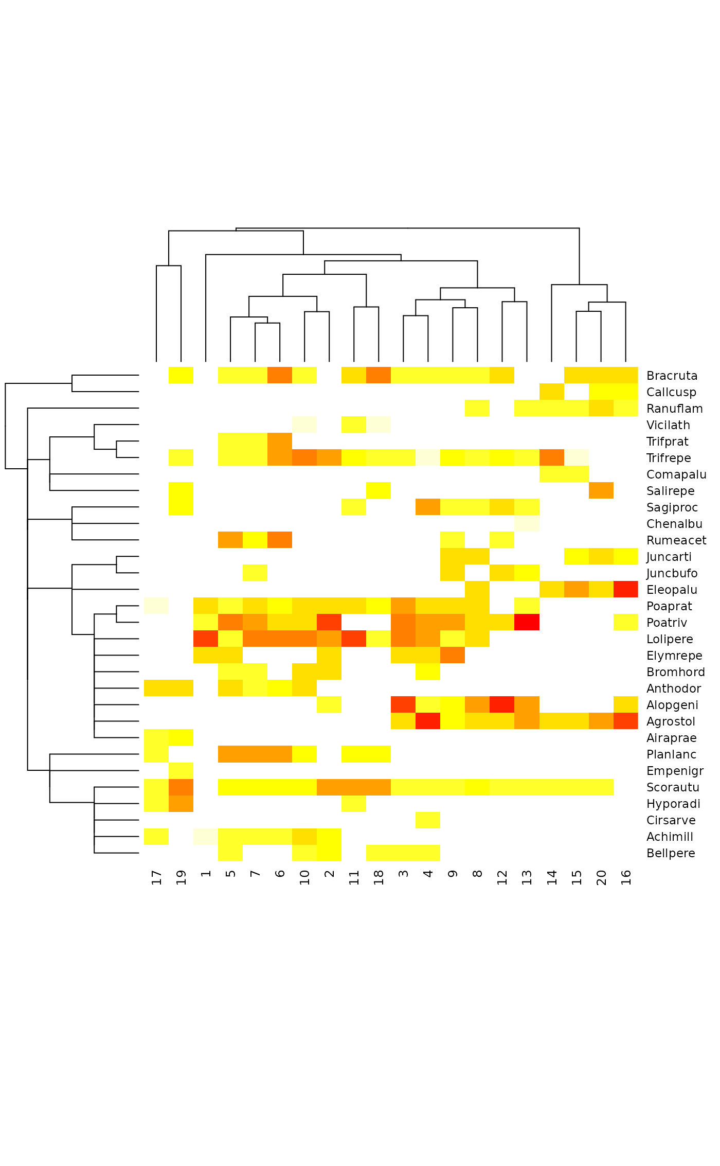
tabasco(dune, plotree, sp.ind = taxontree)

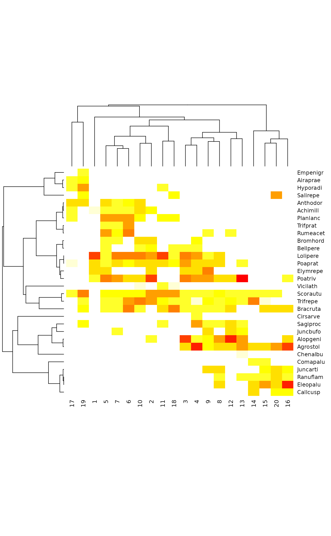
## No reordering of taxonomy
tabasco(dune, plotree, sp.ind = taxontree, Colv = FALSE)

## Species cluster: most dissimilarity indices do a bad job when
## comparing rare and common species, but Raup-Crick makes sense
sptree <- hclust(vegdist(t(dune), "raup"), "average")
tabasco(dune, plotree, sptree)