Multinomial Species Classification Method (CLAM)

The CLAM statistical approach for classifying generalists and specialists in two distinct habitats is described in Chazdon et al. (2011).

Usage

clamtest(comm, groups, coverage.limit = 10, specialization = 2/3, 
   npoints = 20, alpha = 0.05/20)
# S3 method for class 'clamtest'
summary(object, ...)
# S3 method for class 'clamtest'
plot(x, xlab, ylab, main,  pch = 21:24, col.points = 1:4, 
   col.lines = 2:4, lty = 1:3, position = "bottomright", ...)

Arguments

comm: Community matrix, consisting of counts.
groups: A vector identifying the two habitats. Must have exactly two unique values or levels. Habitat IDs in the grouping vector must match corresponding rows in the community matrix comm.
coverage.limit: Integer, the sample coverage based correction is applied to rare species with counts below this limit. Sample coverage is calculated separately for the two habitats. Sample relative abundances are used for species with higher than or equal to coverage.limit total counts per habitat.
specialization: Numeric, specialization threshold value between 0 and 1. The value of \(2/3\) represents ‘supermajority’ rule, while a value of \(1/2\) represents a ‘simple majority’ rule to assign shared species as habitat specialists.
npoints: Integer, number of points used to determine the boundary lines in the plots.
alpha: Numeric, nominal significance level for individual tests. The default value reduces the conventional limit of \(0.05\) to account for overdispersion and multiple testing for several species simultaneously. However, the is no firm reason for exactly this limit.
x, object: Fitted model object of class "clamtest".
xlab, ylab: Labels for the plot axes.
main: Main title of the plot.
pch, col.points: Symbols and colors used in plotting species groups.
lty, col.lines: Line types and colors for boundary lines in plot to separate species groups.
position: Position of figure legend, see legend for specification details. Legend not shown if position = NULL.
...: Additional arguments passed to methods.

Details

The method uses a multinomial model based on estimated species relative abundance in two habitats (A, B). It minimizes bias due to differences in sampling intensities between two habitat types as well as bias due to insufficient sampling within each habitat. The method permits a robust statistical classification of habitat specialists and generalists, without excluding rare species a priori (Chazdon et al. 2011). Based on a user-defined specialization threshold, the model classifies species into one of four groups: (1) generalists; (2) habitat A specialists; (3) habitat B specialists; and (4) too rare to classify with confidence.

Value

A data frame (with class attribute "clamtest"), with columns:

Species:: species name (column names from comm),
Total_*A*:: total count in habitat A,
Total_*B*:: total count in habitat B,
Classes:: species classification, a factor with levels Generalist, Specialist_*A*, Specialist_*B*, and Too_rare.

*A* and *B* are placeholders for habitat names/labels found in the data.

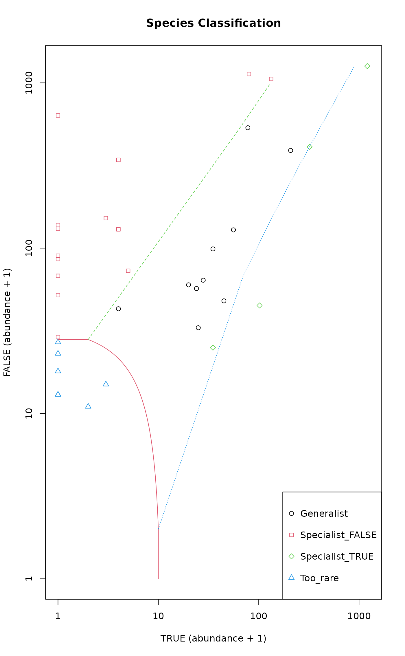
The summary method returns descriptive statistics of the results. The plot method returns values invisibly and produces a bivariate scatterplot of species total abundances in the two habitats. Symbols and boundary lines are shown for species groups.

References

Chazdon, R. L., Chao, A., Colwell, R. K., Lin, S.-Y., Norden, N., Letcher, S. G., Clark, D. B., Finegan, B. and Arroyo J. P.(2011). A novel statistical method for classifying habitat generalists and specialists. Ecology 92, 1332–1343.

Author

Peter Solymos solymos@ualberta.ca

Note

The code was tested against standalone CLAM software provided on the website of Anne Chao (which were then at http://chao.stat.nthu.edu.tw/wordpress); minor inconsistencies were found, especially for finding the threshold for 'too rare' species. These inconsistencies are probably due to numerical differences between the two implementation. The current R implementation uses root finding for iso-lines instead of iterative search.

The original method (Chazdon et al. 2011) has two major problems:

It assumes that the error distribution is multinomial. This is a justified choice if individuals are freely distributed, and there is no over-dispersion or clustering of individuals. In most ecological data, the variance is much higher than multinomial assumption, and therefore test statistic are too optimistic.
The original authors suggest that multiple testing adjustment for multiple testing should be based on the number of points (npoints) used to draw the critical lines on the plot, whereas the adjustment should be based on the number of tests (i.e., tested species). The function uses the same numerical values as the original paper, but there is no automatic connection between npoints and alpha arguments, but you must work out the adjustment yourself.

Examples

data(mite)
data(mite.env)
sol <- with(mite.env, clamtest(mite, Shrub=="None", alpha=0.005))
summary(sol)
#> Two Groups Species Classification Method (CLAM)
#> 
#> Specialization threshold = 0.6666667
#> Alpha level = 0.005
#> 
#> Estimated sample coverage:
#>  FALSE   TRUE 
#> 1.0000 0.9996 
#> 
#> Minimum abundance for classification:
#> FALSE  TRUE 
#>    27     9 
#> 
#>                  Species Proportion
#> Generalist            10      0.286
#> Specialist_FALSE      14      0.400
#> Specialist_TRUE        4      0.114
#> Too_rare               7      0.200
head(sol)
#>   Species Total_FALSE Total_TRUE          Classes
#> 1  Brachy         534         77       Generalist
#> 2    PHTH          89          0 Specialist_FALSE
#> 3    HPAV         389        207       Generalist
#> 4    RARD          85          0 Specialist_FALSE
#> 5    SSTR          22          0         Too_rare
#> 6 Protopl          26          0         Too_rare
plot(sol)