K-means partitioning using a range of values of K

This function is a wrapper for the kmeans function. It creates several partitions forming a cascade from a small to a large number of groups.

Usage

cascadeKM(data, inf.gr, sup.gr, iter = 100, criterion = "calinski",
  parallel = getOption("mc.cores"))

cIndexKM(y, x, index = "all")

# S3 method for class 'cascadeKM'
plot(x, min.g, max.g, grpmts.plot = TRUE, 
     sortg = FALSE, gridcol = NA, ...)

Arguments

data: The data matrix. The objects (samples) are the rows.
inf.gr: The number of groups for the partition with the smallest number of groups of the cascade (min).
sup.gr: The number of groups for the partition with the largest number of groups of the cascade (max).
iter: The number of random starting configurations for each value of \(K\).
criterion: The criterion that will be used to select the best partition. The default value is "calinski", which refers to the Calinski-Harabasz (1974) criterion. The simple structure index ("ssi") is also available. Other indices are available in package cclust. In our experience, the two indices that work best and are most likely to return their maximum value at or near the optimal number of clusters are "calinski" and "ssi".
y: Object of class "kmeans" returned by a clustering algorithm such as kmeans
x: Data matrix where columns correspond to variables and rows to observations, or the plotting object in plot
index: The available indices are: "calinski" and "ssi". Type "all" to obtain both indices. Abbreviations of these names are also accepted.
min.g, max.g: The minimum and maximum numbers of groups to be displayed.
grpmts.plot: Show the plot (TRUE or FALSE).
sortg: Sort the objects as a function of their group membership to produce a more easily interpretable graph. See Details. The original object names are kept; they are used as labels in the output table x, although not in the graph. If there were no row names, sequential row numbers are used to keep track of the original order of the objects.
gridcol: The colour of the grid lines in the plots. NA, which is the default value, removes the grid lines.
...: Other parameters to the functions (ignored).
parallel: Number of parallel processes or a predefined socket cluster. With parallel = 1 uses ordinary, non-parallel processing. The parallel processing is done with parallel package.

Details

The function creates several partitions forming a cascade from a small to a large number of groups formed by kmeans. Most of the work is performed by function cIndex which is based on the clustIndex in package cclust). Some of the criteria were removed from this version because computation errors were generated when only one object was found in a group.

The default value is "calinski", which refers to the well-known Calinski-Harabasz (1974) criterion. The other available index is the simple structure index "ssi" (Dolnicar et al. 1999). In the case of groups of equal sizes, "calinski" is generally a good criterion to indicate the correct number of groups. Users should not take its indications literally when the groups are not equal in size. Type "all" to obtain both indices. The indices are defined as:

calinski:: \((SSB/(K-1))/(SSW/(n-K))\), where \(n\) is the number of data points and \(K\) is the number of clusters. \(SSW\) is the sum of squares within the clusters while \(SSB\) is the sum of squares among the clusters. This index is simply an \(F\) (ANOVA) statistic.
ssi:: the “Simple Structure Index” multiplicatively combines several elements which influence the interpretability of a partitioning solution. The best partition is indicated by the highest SSI value.

In a simulation study, Milligan and Cooper (1985) found that the Calinski-Harabasz criterion recovered the correct number of groups the most often. We recommend this criterion because, if the groups are of equal sizes, the maximum value of "calinski" usually indicates the correct number of groups. Another available index is the simple structure index "ssi". Users should not take the indications of these indices literally when the groups are not equal in size and explore the groups corresponding to other values of \(K\).

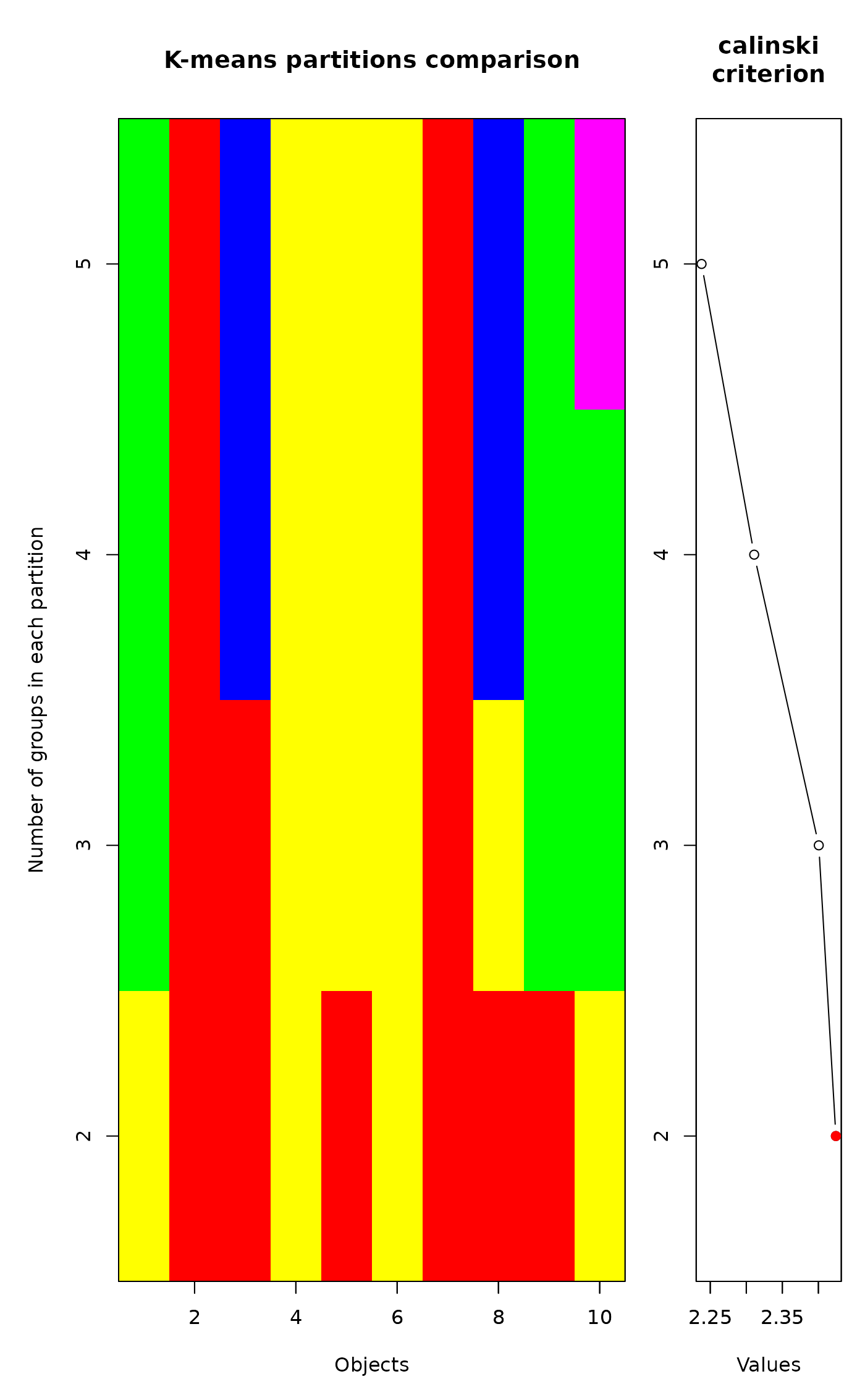
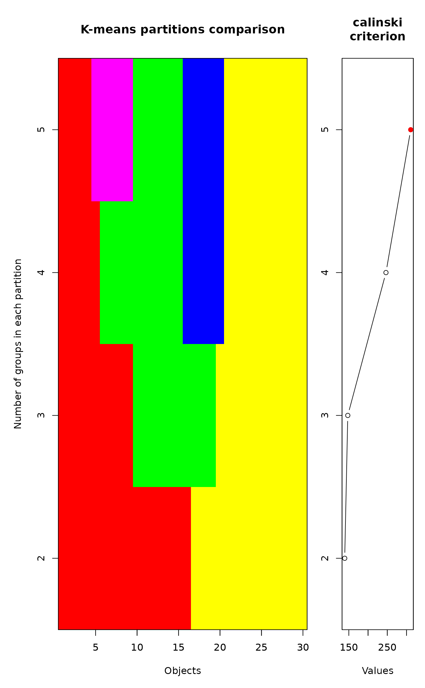
Function cascadeKM has a plot method. Two plots are produced. The graph on the left has the objects in abscissa and the number of groups in ordinate. The groups are represented by colours. The graph on the right shows the values of the criterion ("calinski" or "ssi") for determining the best partition. The highest value of the criterion is marked in red. Points marked in orange, if any, indicate partitions producing an increase in the criterion value as the number of groups increases; they may represent other interesting partitions.

If sortg=TRUE, the objects are reordered by the following procedure: (1) a simple matching distance matrix is computed among the objects, based on the table of K-means assignments to groups, from \(K\) = min.g to \(K\) = max.g. (2) A principal coordinate analysis (PCoA, Gower 1966) is computed on the centred distance matrix. (3) The first principal coordinate is used as the new order of the objects in the graph. A simplified algorithm is used to compute the first principal coordinate only, using the iterative algorithm described in Legendre & Legendre (2012). The full distance matrix among objects is never computed; this avoids the problem of storing it when the number of objects is large. Distance values are computed as they are needed by the algorithm.

Value

Function cascadeKM returns an object of class cascadeKM with items:

partition: Table with the partitions found for different numbers of groups \(K\), from \(K\) = inf.gr to \(K\) = sup.gr.
results: Values of the criterion to select the best partition.
criterion: The name of the criterion used.
size: The number of objects found in each group, for all partitions (columns).

Function cIndex returns a vector with the index values. The maximum value of these indices is supposed to indicate the best partition. These indices work best with groups of equal sizes. When the groups are not of equal sizes, one should not put too much faith in the maximum of these indices, and also explore the groups corresponding to other values of \(K\).

References

Calinski, T. and J. Harabasz. 1974. A dendrite method for cluster analysis. Commun. Stat. 3: 1–27.

Dolnicar, S., K. Grabler and J. A. Mazanec. 1999. A tale of three cities: perceptual charting for analyzing destination images. Pp. 39-62 in: Woodside, A. et al. [eds.] Consumer psychology of tourism, hospitality and leisure. CAB International, New York.

Gower, J. C. 1966. Some distance properties of latent root and vector methods used in multivariate analysis. Biometrika 53: 325–338.

Legendre, P. & L. Legendre. 2012. Numerical ecology, 3rd English edition. Elsevier Science BV, Amsterdam.

Milligan, G. W. & M. C. Cooper. 1985. An examination of procedures for determining the number of clusters in a data set. Psychometrika 50: 159–179.

Weingessel, A., Dimitriadou, A. and Dolnicar, S. 2002. An examination of indexes for determining the number of clusters in binary data sets. Psychometrika 67: 137–160.

Author

Marie-Helene Ouellette Marie-Helene.Ouellette@UMontreal.ca, Sebastien Durand Sebastien.Durand@UMontreal.ca and Pierre Legendre Pierre.Legendre@UMontreal.ca. Parallel processing by Virgilio Gómez-Rubio. Edited for vegan by Jari Oksanen.

Examples

 # Partitioning a (10 x 10) data matrix of random numbers
 mat <- matrix(runif(100),10,10)
 res <- cascadeKM(mat, 2, 5, iter = 25, criterion = 'calinski') 
 toto <- plot(res)

 
 # Partitioning an autocorrelated time series
 vec <- sort(matrix(runif(30),30,1))
 res <- cascadeKM(vec, 2, 5, iter = 25, criterion = 'calinski')
 toto <- plot(res)

 
 # Partitioning a large autocorrelated time series
 # Note that we remove the grid lines
 vec <- sort(matrix(runif(1000),1000,1))
 res <- cascadeKM(vec, 2, 7, iter = 10, criterion = 'calinski')
 toto <- plot(res, gridcol=NA)