Additive Diversity Partitioning and Hierarchical Null Model Testing

In additive diversity partitioning, mean values of alpha diversity at lower levels of a sampling hierarchy are compared to the total diversity in the entire data set (gamma diversity). In hierarchical null model testing, a statistic returned by a function is evaluated according to a nested hierarchical sampling design (hiersimu).

Usage

adipart(...)
# Default S3 method
adipart(y, x, index, weights=c("unif", "prop"),
    relative = FALSE, nsimul=99, method = "r2dtable", ...)
# S3 method for class 'formula'
adipart(formula, data, index=c("richness", "shannon", "simpson"),
    weights=c("unif", "prop"), relative = FALSE, nsimul=99,
    method = "r2dtable", ...)

hiersimu(...)
# Default S3 method
hiersimu(y, x, FUN, location = c("mean", "median"),
    relative = FALSE, drop.highest = FALSE, nsimul=99,
    method = "r2dtable", ...)
# S3 method for class 'formula'
hiersimu(formula, data, FUN, location = c("mean", "median"),
    relative = FALSE, drop.highest = FALSE, nsimul=99,
    method = "r2dtable", ...)

Arguments

y: A community matrix.
x: A matrix with same number of rows as in y, columns coding the levels of sampling hierarchy. The number of groups within the hierarchy must decrease from left to right. If x is missing, function performs an overall decomposition into alpha, beta and gamma diversities.
formula: A two sided model formula in the form y ~ x, where y is the community data matrix with samples as rows and species as column. Right hand side (x) must be grouping variables referring to levels of sampling hierarchy, terms from right to left will be treated as nested (first column is the lowest, last is the highest level). The formula will add a unique indentifier to rows and constant for the rows to always produce estimates of row-level alpha and overall gamma diversities. You must use non-formula interface to avoid this behaviour. Interaction terms are not allowed.
data: A data frame where to look for variables defined in the right hand side of formula. If missing, variables are looked in the global environment.
index: Name of the diversity index, one of "richness" for the number of species, "shannon", "simpson", "invsimpson" of function diversity, "hill1" for Hill number 1 that is the exponent of "shannon", or "hill2" for Hill number 2 that is a synonym of "invsimpson".
weights: Character, "unif" for uniform weights, "prop" for weighting proportional to sample abundances to use in weighted averaging of individual alpha values within strata of a given level of the sampling hierarchy.
relative: Logical, if TRUE then alpha and beta diversity values are given relative to the value of gamma for function adipart.
nsimul: Number of permutations to use. If nsimul = 0, only the FUN argument is evaluated. It is thus possible to reuse the statistic values without a null model.
method: Null model method: either a name (character string) of a method defined in make.commsim or a commsim function. The default "r2dtable" keeps row sums and column sums fixed. See oecosimu for Details and Examples.
FUN: A function to be used by hiersimu. This must be fully specified, because currently other arguments cannot be passed to this function via ....
location: Character, identifies which function (mean or median) is to be used to calculate location of the samples.
drop.highest: Logical, to drop the highest level or not. When FUN evaluates only arrays with at least 2 dimensions, highest level should be dropped, or not selected at all.
...: Other arguments passed to functions, e.g. base of logarithm for Shannon diversity, or method, thin or burnin arguments for oecosimu.

Details

Additive diversity partitioning means that mean alpha and beta diversities add up to gamma diversity, thus beta diversity is measured in the same dimensions as alpha and gamma (Lande 1996). This additive procedure is then extended across multiple scales in a hierarchical sampling design with $i = 1, 2, 3, \ldots, m$ levels of sampling (Crist et al. 2003). Samples in lower hierarchical levels are nested within higher level units, thus from $i=1$ to $i=m$ grain size is increasing under constant survey extent. At each level $i$, $\alpha_i$ denotes average diversity found within samples.

At the highest sampling level, the diversity components are calculated as $$\beta_m = \gamma - \alpha_m$$ For each lower sampling level as $$\beta_i = \alpha_{i+1} - \alpha_i$$ Then, the additive partition of diversity is $$\gamma = \alpha_1 + \sum_{i=1}^m \beta_i$$

Average alpha components can be weighted uniformly (weight="unif") to calculate it as simple average, or proportionally to sample abundances (weight="prop") to calculate it as weighted average as follows $$\alpha_i = \sum_{j=1}^{n_i} D_{ij} w_{ij}$$ where $D_{ij}$ is the diversity index and $w_{ij}$ is the weight calculated for the $j$th sample at the $i$th sampling level.

The implementation of additive diversity partitioning in adipart follows Crist et al. 2003. It is based on species richness ($S$, not $S-1$), Shannon's and Simpson's diversity indices stated as the index argument.

The expected diversity components are calculated nsimul times by individual based randomisation of the community data matrix. This is done by the "r2dtable" method in oecosimu by default.

hiersimu works almost in the same way as adipart, but without comparing the actual statistic values returned by FUN to the highest possible value (cf. gamma diversity). This is so, because in most of the cases, it is difficult to ensure additive properties of the mean statistic values along the hierarchy.

Value

An object of class "adipart" or "hiersimu" with same structure as oecosimu objects.

References

Crist, T.O., Veech, J.A., Gering, J.C. and Summerville, K.S. (2003). Partitioning species diversity across landscapes and regions: a hierarchical analysis of $\alpha$, $\beta$, and $\gamma$-diversity. Am. Nat., 162, 734–743.

Lande, R. (1996). Statistics and partitioning of species diversity, and similarity among multiple communities. Oikos, 76, 5–13.

Author

Péter Sólymos, solymos@ualberta.ca

Examples

## NOTE: 'nsimul' argument usually needs to be >= 99
## here much lower value is used for demonstration

data(mite)
data(mite.xy)
data(mite.env)
## Function to get equal area partitions of the mite data
cutter <- function (x, cut = seq(0, 10, by = 2.5)) {
    out <- rep(1, length(x))
    for (i in 2:(length(cut) - 1))
        out[which(x > cut[i] & x <= cut[(i + 1)])] <- i
    return(out)}
## The hierarchy of sample aggregation
levsm <- with(mite.xy, data.frame(
    l1=1:nrow(mite),
    l2=cutter(y, cut = seq(0, 10, by = 2.5)),
    l3=cutter(y, cut = seq(0, 10, by = 5)),
    l4=rep(1, nrow(mite))))
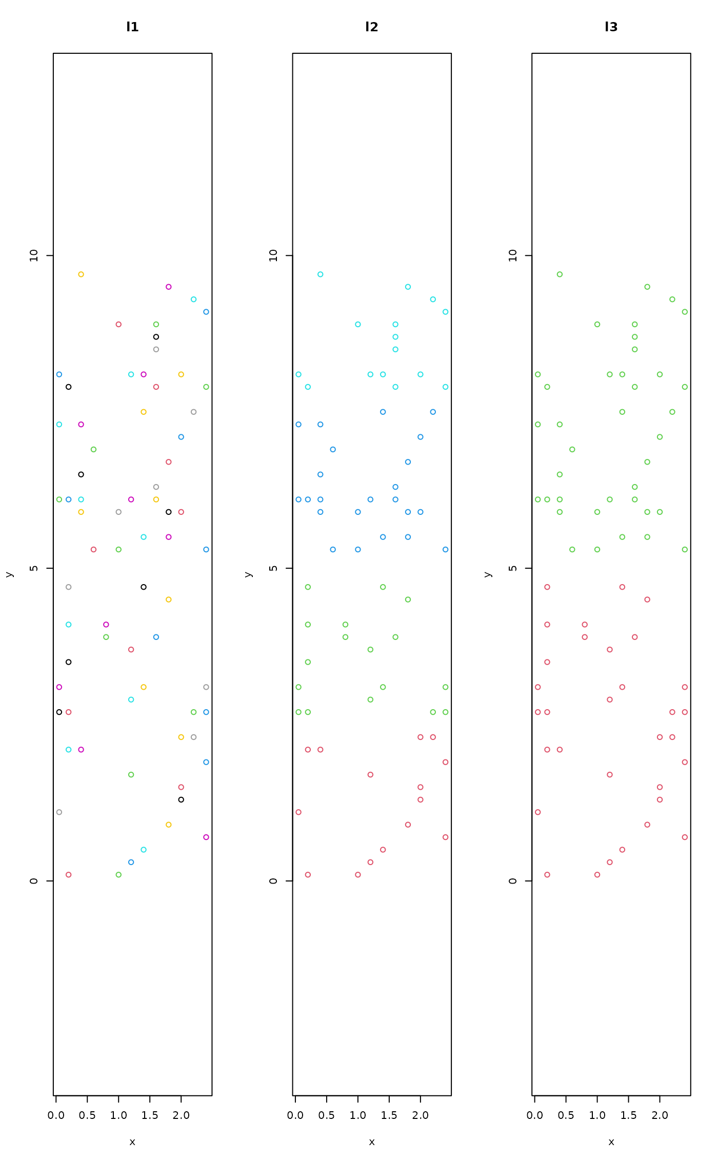
## Let's see in a map
par(mfrow=c(1,3))
plot(mite.xy, main="l1", col=as.numeric(levsm$l1)+1, asp = 1)
plot(mite.xy, main="l2", col=as.numeric(levsm$l2)+1, asp = 1)
plot(mite.xy, main="l3", col=as.numeric(levsm$l3)+1, asp = 1)

par(mfrow=c(1,1))
## Additive diversity partitioning
adipart(mite, index="richness", nsimul=19)
#> adipart object
#> 
#> Call: adipart(y = mite, index = "richness", nsimul = 19)
#> 
#> nullmodel method ‘r2dtable’ with 19 simulations
#> options:  index richness, weights unif
#> alternative hypothesis: statistic is less or greater than simulated values
#> 
#>         statistic     SES   mean   2.5%    50%  97.5% Pr(sim.)  
#> alpha.1    15.114 -34.264 22.379 22.027 22.414 22.695     0.05 *
#> gamma      35.000   0.000 35.000 35.000 35.000 35.000     1.00  
#> beta.1     19.886  34.264 12.621 12.305 12.586 12.973     0.05 *
#> ---
#> Signif. codes:  0 ‘***’ 0.001 ‘**’ 0.01 ‘*’ 0.05 ‘.’ 0.1 ‘ ’ 1
## the next two define identical models
adipart(mite, levsm, index="richness", nsimul=19)
#> adipart object
#> 
#> Call: adipart(y = mite, x = levsm, index = "richness", nsimul = 19)
#> 
#> nullmodel method ‘r2dtable’ with 19 simulations
#> options:  index richness, weights unif
#> alternative hypothesis: statistic is less or greater than simulated values
#> 
#>         statistic      SES     mean     2.5%      50%   97.5% Pr(sim.)  
#> alpha.1    15.114 -35.7223 22.32707 22.01143 22.37143 22.6214     0.05 *
#> alpha.2    29.750 -24.5658 34.89474 34.36250 35.00000 35.0000     0.05 *
#> alpha.3    33.000   0.0000 35.00000 35.00000 35.00000 35.0000     0.05 *
#> gamma      35.000   0.0000 35.00000 35.00000 35.00000 35.0000     1.00  
#> beta.1     14.636   8.6481 12.56767 12.17571 12.52857 12.9757     0.05 *
#> beta.2      3.250  15.0159  0.10526  0.00000  0.00000  0.6375     0.05 *
#> beta.3      2.000   0.0000  0.00000  0.00000  0.00000  0.0000     0.05 *
#> ---
#> Signif. codes:  0 ‘***’ 0.001 ‘**’ 0.01 ‘*’ 0.05 ‘.’ 0.1 ‘ ’ 1
adipart(mite ~ l2 + l3, levsm, index="richness", nsimul=19)
#> adipart object
#> 
#> Call: adipart(formula = mite ~ l2 + l3, data = levsm, index =
#> "richness", nsimul = 19)
#> 
#> nullmodel method ‘r2dtable’ with 19 simulations
#> options:  index richness, weights unif
#> alternative hypothesis: statistic is less or greater than simulated values
#> 
#>         statistic     SES     mean     2.5%      50%   97.5% Pr(sim.)  
#> alpha.1    15.114 -47.873 22.42556 22.16429 22.41429 22.6857     0.05 *
#> alpha.2    29.750 -33.466 34.86842 34.61250 35.00000 35.0000     0.05 *
#> alpha.3    33.000   0.000 35.00000 35.00000 35.00000 35.0000     0.05 *
#> gamma      35.000   0.000 35.00000 35.00000 35.00000 35.0000     1.00  
#> beta.1     14.636  12.095 12.44286 12.02893 12.47143 12.6539     0.05 *
#> beta.2      3.250  20.389  0.13158  0.00000  0.00000  0.3875     0.05 *
#> beta.3      2.000   0.000  0.00000  0.00000  0.00000  0.0000     0.05 *
#> ---
#> Signif. codes:  0 ‘***’ 0.001 ‘**’ 0.01 ‘*’ 0.05 ‘.’ 0.1 ‘ ’ 1
## Hierarchical null model testing
## diversity analysis (similar to adipart)
hiersimu(mite, FUN=diversity, relative=TRUE, nsimul=19)
#> hiersimu object
#> 
#> Call: hiersimu(y = mite, FUN = diversity, relative = TRUE, nsimul = 19)
#> 
#> nullmodel method ‘r2dtable’ with 19 simulations
#> 
#> alternative hypothesis: statistic is less or greater than simulated values
#> 
#>         statistic     SES    mean    2.5%     50%  97.5% Pr(sim.)  
#> level_1   0.76064 -71.055 0.93877 0.93372 0.93887 0.9424     0.05 *
#> leve_2    1.00000   0.000 1.00000 1.00000 1.00000 1.0000     1.00  
#> ---
#> Signif. codes:  0 ‘***’ 0.001 ‘**’ 0.01 ‘*’ 0.05 ‘.’ 0.1 ‘ ’ 1
hiersimu(mite ~ l2 + l3, levsm, FUN=diversity, relative=TRUE, nsimul=19)
#> hiersimu object
#> 
#> Call: hiersimu(formula = mite ~ l2 + l3, data = levsm, FUN = diversity,
#> relative = TRUE, nsimul = 19)
#> 
#> nullmodel method ‘r2dtable’ with 19 simulations
#> 
#> alternative hypothesis: statistic is less or greater than simulated values
#> 
#>      statistic      SES    mean    2.5%     50%  97.5% Pr(sim.)  
#> unit   0.76064  -71.178 0.93851 0.93396 0.93906 0.9420     0.05 *
#> l2     0.89736 -131.398 0.99801 0.99698 0.99783 0.9993     0.05 *
#> l3     0.92791 -507.053 0.99937 0.99911 0.99935 0.9996     0.05 *
#> all    1.00000    0.000 1.00000 1.00000 1.00000 1.0000     1.00  
#> ---
#> Signif. codes:  0 ‘***’ 0.001 ‘**’ 0.01 ‘*’ 0.05 ‘.’ 0.1 ‘ ’ 1
## Hierarchical testing with the Morisita index
morfun <- function(x) dispindmorisita(x)$imst
hiersimu(mite ~., levsm, morfun, drop.highest=TRUE, nsimul=19)
#> hiersimu object
#> 
#> Call: hiersimu(formula = mite ~ ., data = levsm, FUN = morfun,
#> drop.highest = TRUE, nsimul = 19)
#> 
#> nullmodel method ‘r2dtable’ with 19 simulations
#> 
#> alternative hypothesis: statistic is less or greater than simulated values
#> 
#>    statistic     SES      mean      2.5%       50%   97.5% Pr(sim.)  
#> l1   0.52070  4.4807  0.355380  0.289890  0.352507  0.4182     0.05 *
#> l2   0.60234 10.3325  0.164149  0.099261  0.158335  0.2428     0.05 *
#> l3   0.67509 19.0025 -0.195318 -0.254971 -0.204844 -0.1069     0.05 *
#> ---
#> Signif. codes:  0 ‘***’ 0.001 ‘**’ 0.01 ‘*’ 0.05 ‘.’ 0.1 ‘ ’ 1